Who lends to the Indian state?

by Aneesha Chitgupi, Ajay Shah, Manish Kumar Singh, Susan Thomas and Harsh Vardhan.

Public finance researchers in India have paid great attention to debt and deficits. By now, the main messages of the field have started sinking into common knowledge: that it is good to run primary deficits in most years, so as to create space to surge the deficit once in a while when faced with a crisis. There is an adjacent field of public debt management that is equally important. Here, the strategic question is: How should the government borrow? From whom? Debt management strategy has not received the required level of interest.

Strategic thinking in debt management

A sound public debt management strategy must cater to three objectives:

• The mechanism for borrowing must not induce economic distortions upon the domestic economy.
• It must create strategic depth of being able to borrow on a very large scale when faced with great challenges, once every few decades.
• It must induce sustainable mechanisms for reasonably low cost borrowing, at reasonably predictable rates, for the long term.

There are four main pathways to choose from in debt issuance:

1. Monetisation of the deficit. Here, the central bank distorts the monetary base with `fiscal dominance’ where it buys the bonds issued by the government.
2. Coerced borrowing from financial firms. These are typically regulated firms, who are coerced using the tools of financial regulation.
3. Borrowing from voluntary participants (domestic or foreign). This is done through local currency bonds issued domestically, possibly nominal and possibly inflation indexed.
4. Borrowing abroad using foreign currency denominated bonds. As an example, this could involve Yen denominated bonds issued in London.

As with many other countries, we started out in India with the first method (monetisation of the deficit). This induces an economic distortion: the loss of monetary policy autonomy. A long journey of monetary policy reform took place, from the Ways and means agreement of 1993, to the Monetary policy framework agreement in 2015 that ushered in inflation targeting. This freed up monetary policy from the limitations imposed by debt management. In 2015, there was an attempt at institutional reform, in the form of the establishment of the Public Debt Management Agency (freeing up the Reserve Bank of India of the responsibility of issuing public debt), but this did not come to pass.

From 1993 onward, the main strategy for public debt management in India has involved method 2 in the list: a system of `financial repression’ where the government borrows from coerced financial firms. This is a tax upon financial intermediation. The interest rates discovered through government borrowing are important prices that impinge upon the economy. But these rates are distorted owing to the presence of coerced buyers of government debt. The lack of voluntary lenders creates the lack of strategic depth. The government is limited in how it can expand its borrowing when faced with special situations.

From the late 1990s onwards, economists and thinkers have sought to enhance fiscal prudence in India through the mechanism of fiscal responsibility law. It is increasingly clear that this does not work. In recent work, Datta et. al. 2023 show that the Indian constitutional arrangements frustrate the possibility of Parliamentary law imposing fiscal discipline upon the union government. Once this idea is internalised, there is one main path towards fiscal responsibility: market discipline. This requires removing the system of financial repression.

Who lends to the Indian state?

In this context, the question Who lends to the Indian state? attains importance. A recent paper by Aneesha Chitgupi, Ajay Shah, Manish Singh, Susan Thomas and Harsh Vardhan examines this question. For a period of 10 years, we assemble information from multiple sources, which were all available in the public domain, to examine the nature of lenders to the Indian state. Some discoveries that we make are:

• The SLR went down in the last decade. This meant that the extent of bank funds mandated for the government decreased. However, the actual investments by banks in government debt securities was higher than what was mandated.
• Simultaneously, there was major growth in the role of insurance and pension funds lending to the government. While de jure financial repression of banks declined, there has been no such retreat with pensions and insurance.
• All the three groups of financial firms bought a lot more government bonds as compared with the de jure requirements. Excess ownership went from about 0 in 2011 to Rs.30 trillion in 2021.
• How did the government increase borrowing over the last decade, while simultaneously elongating the maturity profile? The answer lies in (a) Strong growth in insurance and pensions industries, and (b) Excess ownership of government bonds by coerced industries.
• The voluntary lenders are the private firms, MFs and FIIs, who are 4.8% of investors in the government debt market for 2021. India (along with China) remains an outlier in having very low borrowing from international debt markets.

Important questions for the future

This field is target rich with interesting questions, some of which are:

1. Why do financial firms lend so much to the government?
2. What will the structure of lenders to the government look like, 10 years out into the future?
3. If a big surge in borrowing is required, where will it come from?
4. How are households and firms changing their behaviour in response to the financial repression tax?
5. What is the path to fiscal responsibility?

Conclusion

The field of public finance in India has studied deficits and debt. There has been work on the institutional arrangements for debt management (i.e. the establishment of the Public Debt Management Agency). There has been relatively little work on the economic reasoning, the strategic thinking for debt management. In this paper, we offer novel insights and facts for this journey. More research is required, at the interfaces between public finance, finance and public administration, to grow knowledge on the important field of debt management strategy.

How "Orderly" is the Evolution of the Indian Yield Curve?

by Harsh Vardhan.

"Financial market stability and the orderly evolution of the yield curve are public goods and both market participants and the RBI have a shared responsibility in this regard."

Shaktikanta Das, Governor, RBI, October 2020

"Right from October 2020, we have given explicit guidance to the bond market. We expect an orderly evolution of the yield curve, it cannot be otherwise,"

Shaktikanta Das, Governor, RBI, February 2021

As the Covid pandemic has ebbed, central banks across the world are withdrawing the extra-ordinary easy monetary policy that was followed by them since the onset of the pandemic. Reserve Bank in India (RBI) is no exception. A week ago, it took the extra ordinary step of convening an ad-hoc meeting of the monetary policy committee (MOC) to hike the policy interest rates by 40 basis points and also increase the cash reserve ratio (CRR) for banks to take out liquidity from the banking system.

As this “normalisation” of the monetary policy unfolds, its impact on the financial stability has become a matter of concern. The statements of the RBI Governor quoted above, reflect the concern RBI has on financial stability and the evolution of the yield curve. While financial stability is a broad, all encompassing term, evolution of the yield curve is a much more specific idea that can potentially be objectively assessed. In this article I try to assess the orderliness of the evolution of the yield curve over the last four years.

Yield curve describes the basis interest structure in the economy. As the central bank takes policy actions bonds markets reprice the yields and the shape of the yield curve changes. As a fundamental input to pricing of a wide array of assets, predictable and orderly evolution of the yield curve is indeed desirable. High volatility and unpredictability in the evolution of the yield curve, especially when the policy actions taken to normalise monetary policy and regain the GDP growth trajectory post the pandemic, could result in mispricing of financial assets. RBIs concerns and expectation of such orderly evolution are understandable.

In this article, I try to assess the orderliness of evolution of the yield curve. I use data on the yield curve for the 4-year period of 1 April 2018 to 10 May 2022 to empirically assess how the yield curve has changed during this period. To be clear, this article does not evaluate the merits of the RBI’s intent or efforts at managing the yield curve; it only attempts to empirically assess how the yield curve has behaved over this period.

Assessing the evolution of the yield curve:

While it is easy to understand why policy makers would want the yield to evolve in an “orderly” manner in response to policy actions, it is not very easy to define what exactly an orderly evolution means. Trading in government securities takes place every day where all types of financial institutions participate. Even the RBI, through its treasury operations and open market operations participates in the government bond market. The collective actions of all these players determine the prices of government bonds and hence the yield on them.

We could hypothesise orderly evolution to mean that the daily changes in the yields across the curve are smooth and stable. There are two parameters we can look at the describe such smooth and orderly evolution – the volatility of daily yield change and the correlation of changes in yields across varying maturities. If the volatility of daily change in yields remains low and the correlation of yield changes across maturities is high, then it would mean that the yield curve is moving with the policy rates, in a non-disruptive and predictable manner. Such a yield curve can be considered as evolving orderly. On the other hand, increased volatility of daily change and reduced correlation would signal increase in the “disorder” in the evolution of the yield curve.

Data and analysis:

The data for this analysis is the daily yields data on the 3 month treasury bills (T Bills), 1 year, 3, year, 5 year, and 10 year maturity government securities (GoI securities) from 01 April 2018 to 10 May 2022, a total of 993 trading days of data obtained from Bloomberg. Of these maturities the 10-year securities are the most liquid and provide data for every trading day. For the other securities there are days where there would be no trading and hence no data would be available. We consider the previous days yield to continue for such non trading days which means that the change in yields for such days is considered to be zero.

For the purpose of my analysis, I divide the data into 4 time periods as follows:

The first period is from 1 April 2018 to 11 February 2019 which can be called the "pre low interest rate" period. RBI started cutting policy rates from February 19 up until May of 2020. Hence this is the period of stable policy rates. This period has data for 215 trading days.

The second period is from 19 February 2019 to 31 October 2020 is the "downward policy rates and pandemic period" when policy rates were reduced regularly to hit the lowest rate of 4% of repo by May 2020. I extend the period to Oct 31,2020 as RBI clearly started focusing on orderly evolution from October onwards. This period gives us data on 411 trading days.

The third period is from 01 November 2020 to 31 December 2021 which starts with the date of RBI publicly announced its focus on orderly evolution of the yield curve and ends with roughly the end of the pandemic and the reopening of the economy. While the end date is admittedly somewhat arbitrary it coincides with global trend towards rising rates that started in January 2022. This period gives us data on 282 trading days.

The fourth and the shorted period is from 01 January 2022 to 10 May 2022 is the last period where Indian interest rates started inching up (along with interest rates across the world). It includes a few days of data post the surprise, out of turn policy rate hike in May 2022. This period has data on 85 trading days.

For each of these four periods, I compute the following:

• Daily change in the yields of each of the four maturity GoI securities.
• Average daily yield change and the standard deviation of the change in the daily yield which I use as the measure of volatility of the daily change.
• Correlation between yield changes of these 4 GoI securities.

Results:

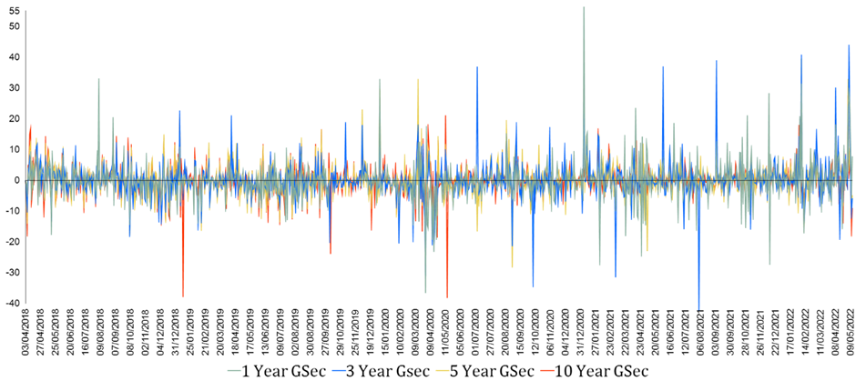
Figure 1 below presents a chart of the daily yield change in these 4 securities over this entire period of little over 4 years and 993 trading days.

Figure 1: Daily Change in Yields on GoI Securities in Basis Points

Source: Bloomberg, author’s analysis

Overall, the chart shows that the volatility of the daily change seems to go up with the onset of Covid in March 2020 with larger and more frequent spikes. This is especially true for the lower maturity; the 3 year and the 1 year maturity securities.

In order to understand the trends in the pattern of the daily change in yield, I plot the 30-day moving average of the daily change in yield as presented in Figure 2 below.

Figure 2: 30 Day Moving Average of Daily Change in Yields on GoI Securities in Basis Points

Source: Bloomberg, author’s analysis

Figure 2 clearly shows a pattern in the changes in the yield curve. The first period has much smaller change daily change in the curve and the changes across maturities are fairly highly correlated. The second period shows much more volatility in the daily change and a significant reduction in the correlation between yield change across maturity. This volatility comes down in the third period and the correlation improves, probably as an outcome of RBIs repeated exhortations and possibly actions in the bond market. The last period shows further reduction in volatility but the correlation is still lower than in the first period indicating that RBIs notices to the bond market and actions have had some success.

In order to more concretely understand the volatility and correlations across these periods, next two charts present the mean daily change in yields and the volatility of the daily change measured as the standard deviation of the daily change in yield.

Figure 3: Mean Daily Change in Yields on GoI Securities

Source: Bloomberg, author’s analysis

This chart clearly describes the interest rate trends in these four periods. The first period had, by and large, stable yield curve with very small changes in yields. The second period shows a secular decline in interest rates across all maturities in response to policy rate changes. The third period shows a reversal of trends and modest rise of interest rates ie the upward movement of the yield curve which becomes much more pronounced and sharper in the fourth period.

Figure 4: Volatility of Daily Change in Yields on GoI Securities

Source: Bloomberg, author’s analysis

This chart shows that the volatility of yield changes has indeed gone up noticeably in the third period when the overall rates showed an increase. The volatility increased especially for the shorter maturity papers – 1 year and 3-year maturity. This probably is the basis of the RBIs focus on ‘orderly’ evolution and hints to the bond market of its discomfort with high volatility. The fourth period shows that the elevated volatility has persisted which means that the bond market has responded only modestly to the RBI’s exhortations. Another important feature to note is that the volatility of the 10 year and the 5 year maturity securities has been contained in the third and the fourth period while that of the shorter maturity securities has continued to remain high. This possibly could also be due to RBI’s targeted interventionsh in the bond market to contain the rise and volatility of yields on long term securities.

Finally, I look at the correlations of yield changes across these maturities. Table below presents the correlation matrix of the four periods.

Table: Correlation Matrix for Yield Change in GoI Securities of Varying Maturities

Source: Bloomberg, author’s analysis

The correlation matrix shows high correlations between yield changes in the first period that start going down in the second period and decline precipitously in the third period. While they improve in the fourth period, they are still below the high levels of the first period. Clearly, the yield curve moved more haphazardly in the third period with high volatility and low correlation between yield changes across maturities. The fourth period shows improvement in correlations probably due to RBIs constant notices to the bond market (and its possible interventions in the market), they do not reach the levels of the first halcyon period.

Conclusion:

This data shows that RBI concern on orderly evolution of yield curve is well placed. The data clearly shows that in period 2, as the policy rates came down, the yield curve volatility shot up. It may well be that the RBI’s focus during this time was on keeping the long-term interest rates low to facilitate economic recovery during the pandemic. The bond market, on the other hand, was concerned about the economic impact of the pandemic and resulting tussle between the RBI and bond market participants actions resulted in increased volatility and break down of correlations in yield movements across maturity. RBI became aware of this volatility towards the third quarter of fiscal 2022 and realised that low rates will not be enough for economic recovery and the excess volatility must be curbed. As it started expressing its desire of an orderly evolution (accompanied possibly by market interventions) there was a modest decline in volatility and improvement in correlations. However, the markets are still not anywhere close to the halcyon pre-pandemic period.

Harsh Vardhan is an independent management consultant and researcher based in Mumbai. The author thanks Surbhi Bhatia for research assistance, and Josh Felman and anonymous referees for very useful comments

A cooperative liquidity window for mutual funds: A debate

by Harsh Vardhan vs. Josh Felman and Ajay Shah.

Problem statement

There is a mismatch between the growth of the mutual fund industry versus the maturation of the financial markets (Shah, 2018). This generated trouble after the IL&FS default of August 2018, and will likely make trouble in the future also. Mutual funds are in an awkward place, promising liquidity to their customers but lacking a liquid bond market. Some years ago, the exchanges were getting better, and there was a path to building the Bond-Currency-Derivatives Nexus, so we could hope that progress on both paths would come along and solve the problem of the mutual funds. Now, both elements (exchanges and bond market reform) have a weak outlook. Is there a way out of this conundrum? Can a liquidity window for mutual funds be created, through which the problem of the mutual funds can be solved?

Why we need this and how it can work, by Harsh Vardhan

Indian debt mutual funds have grown rapidly over the past few years. Debt funds got a strong push after demonetisation. Currently the total assets under management (AuM) of debt funds are ~ Rs 15 Trn. There are individual debt fund schemes with AuMs of over Rs 1 Trn.

Debt funds invest their corpus in debt securities. In India there are two main classes of debt securities – those issued by the government including central and state governments and those issued by companies. Both have very poor liquidity. In the case of government bonds, while there is a somewhat liquid interbank market, a large part of the liquidity is in a single ‘benchmark’ paper which is typically a 10 year bond. When a new 10 year bond is issued, the old one ceases to be the benchmark and its liquidity drops sharply. The lack of liquidity is even worse with corporate bonds.

Most debt mutual funds promise high liquidity to their investors. For liquid and short duration funds, redemption proceeds are credited to the investor on T+1 while for most other debt funds it is T+2. MFs suffer the agony of liquid liabilities and illiquid assets. They manage this challenge through two pathways: (a) holding cash (typically less than 5% of AuM) and (b) having credit lines from banks.

There is considerable systemic risk in the Indian financial system, and situations where these two pathways prove to be inadequate. As an example, Franklin Templeton shut down six debt schemes when redemptions were unusually large and the bond market was unusually illiquid. The redemption pressure that they faced had nothing to do with their money management; it was induced by an episode of systemic risk.

In the anatomy of these recurrent debt market crises, one interesting feature is market failure in the form of a negative externality. Purely at random, when large redemptions show up at any one door, the selling that this induces drives down prices (as the overall market is illiquid and impact cost is high), which adversely impacts the NAV of all other funds. For any rational economic agent that sees the first inkling of higher outflows (either by watching flows or by looking at NAV changes), it is rational to yank all debt investments. This creates a channel through which selling by one fund induces redemptions for others.

Another way to locate these problems in the framework of market failure is to see that market liquidity is a public good. As an example, the liquidity of Nifty futures is non-rival (your consumption of liquidity does not adversely impinge on my access to liquidity) and non-excludable (everyone can access the Nifty futures market). When we build liquid markets, we are creating a public good.

All market failure is ultimately a problem of coordination between economic agents. We should look for collective action through which some of the problems of debt mutual funds can be addressed.

There are two solutions going around, for this problem of bond market illiquidity, which just don’t make sense. One strategy is for regulators to demand that mutual funds hold more capital. Mutual funds are not balance-sheet based entities and the journey of trying to amplify their equity capital requirements is conceptually wrong. Another strategy is for the central bank or the government through any other agency, to run a liquidity window for mutual funds. When the full consequences of this play out for mutual funds, it is likely to leave them worse off.

Is there a way out of this jam? I believe we can establish a Cooperative Liquidity Window (CLW), built by mutual funds for mutual funds -- with a small involvement of the state -- which can help solve this problem. For the people who are too used to state leadership in such things, we should point out that the Bank of England played this kind of function -- liquidity support for distressed banks -- for centuries as a purely private organisation; it was only nationalised in 1946. During the great depression in the US in the 1930s, J P Morgan, founder owner of the eponymous bank, orchestrated a bail-out of the American banking system through co-operative efforts of larger, stronger banks. These experiences are food for thought, and the design proposed here draws on this history.

For such an emergency liquidity support mechanism, we should establish five conceptual objectives:

• It should use no public money.
• There should be an extremely low amount of state coercion involved, in getting some MFs to participate in the CLW, and no role for the state in terms of regulation, management, appointments, or rule-making of the CLW.
• The governance of the mechanism should be within the AMCs that participate in it; it should operate as a self regulatory organisation.
• The capital to set up and operate the mechanism should be provided by the participants; it should operate as a mutual co-operative; rules of access to the mechanism should be defined by the participants.
• It should be only an emergency liquidity support system. The criteria for defining an emergency, and the extent of support that can be provided to individual entities, should be defined by members as the by-laws of the mechanism.

How would the proposed CLW work?

1. The participating AMCs would create a vehicle by contributing to the equity of the vehicle. The vehicle could be set up as a trust or any other legal form that minimizes transaction costs.
2. Some members would be coerced by SEBI (the largest firms adding up to perhaps 75% of the category AUM) and others would be voluntary participants (those who would like to benefit from its services even if not forced by SEBI). Apart from this, there would be no role for the state power in the CLW, in any fashion.
3. The equity contribution of each MF should be determined by its debt fund corpus. For example, all MFs with debt fund AuM of over Rs 1 Trn might contribute Rs.5 Billion, those with an AuM of Rs 0.5 Trn to 1 Trn might contribute Rs. 3 Billion, and so on. The CLW governance must write the specific rules of equity contributions.
4. The CLW would leverage up and create a corpus that supports a securities repurchase (repo) operation in the event of stress.
5. When a member AMC faces severe redemption pressure (way beyond what is deemed normal by the members collectively as defined by the governance rule of the CLW) it would pledge its eligible debt securities to raise short term liquidity. This would be akin to a bank accessing the repo window in the event of a run.
6. This window would also accept liquidity from members like a normal repo window.
7. The rules regarding the extent of liquidity support provided, the tenure, the bid-ask spread, acceptable securities as collateral and hair cuts, etc. would all be defined by the members collectively.
8. The CLW would operate as a not for profit entity or provide a modest return on equity to the member shareholders.

Currently there are ~45 AMCs in India. If we assume that 40 of them participate, each contributing an average of Rs 1 billion of equity capital, we would have Rs.40 billion of equity capital in hand. Assuming 4x leverage, the resources of the organisation would be Rs.160 billion. It is easy to go to much higher values.

The CLW should support participating MFs only in dealing with liquidity issues and not credit risk issues. This should be enshrined in the governance and operating rules of the CLW. Considering that the CLW will be managed by the AMCs themselves, who are all deeply informed players, it is reasonable to assume that they will be able to differentiate between liquidity and credit issues, Further, at a security level, the CLW will determine eligibility of securities and haircuts applicable. This will ensure that even in providing liquidity support, credit issues are not ignored. The rules of operation of the CLW should be well known, ex ante, so all the participating MFs face a predictable environment.

Let us simulate how the Franklin Templeton crisis might have played out, if this CLW was in place. The issues faced by Franklin Templeton’s shuttered debt funds schemes were purely liquidity issues: Over the last 18 months or so, they have returned upwards of 90% of the AUM at the time of shutting the schemes. Further, the return on these funds during the time was comparable with other funds in the same asset class. As the Franklin Templeton crisis was a liquidity crisis and not a credit crisis, the CLW would have been in play to support the liquidity crisis at Franklin Templeton. With illustrative assets of Rs.160 billion, it would have had the financial depth to deal with this situation, where all six affected funds put together had a total AUM of about Rs. 250 billion.

This design is not a substitute for a deep and developed bond market. A liquid market for securities is always the best solution to deal with any liquidity issues. But we face a problem today: We have a situation where the debt mutual funds corpus has grown very significantly and yet the bond market, especially the corporate bond market, remains very illiquid. The CLW is a mechanism where enlightened self interest can create a cooperative which helps the sector deal with a dangerous liquidity challenge.

In my proposal, there is only one use of state power: I feel SEBI should force large debt funds adding up to (say) 75% of the industry AUM to be members of the CLW, and force non-members to communicate this lack of membership in their customer-facing communications. The justification for this use of state power lies in the extent to which this would help reduce systemic risk (innocent bystanders being adversely affected in the next mutual fund crisis). This coercion addresses the free rider problem, where any one MF may derive benefits from the more stable mutual fund / bond market system, but try to be stingy in not paying for this stabilisation. Apart from this, I propose there should be no state involvement / control / regulation of the analysis, design, staffing, rule-making or operation of the CLW.

All members would have the self interest of making the facility work well -- as they are both owners and customers -- and they would thus exert governance. This is a problem where a cooperative solution works well. There is no market failure in the working of the CLW, and thus no role for regulation or any other involvement of the state.

There is one limitation in this design. The CLW will not be adequate if there is a full fledged financial crisis, such as what was experienced in 2008. In that case, the CLW would become one more element of the financial system that would have to be analysed in the crisis management at MOF.

There is no solution which can cover up for the lack of a bond market, by Josh Felman and Ajay Shah

Bond mutual funds are facing a serious dilemma. On the one hand, they promise investors liquidity, the ability to withdraw money at short notice. But on the other hand, they hold assets that are largely illiquid and difficult to sell. As a result, they face a mismatch between what they promise and what they can actually deliver.

Investors typically pay little attention to this mismatch, because most of the time it isn’t apparent. That’s because on most normal days, the investors who want to withdraw their money are more than counterbalanced by the many investors who are putting their money into the funds. It is only when this balance is disrupted, when a large proportion of investors “run” to take their money out, that mutual funds must sell their assets and the liquidity mismatch is revealed (Sane, Shah, Zaveri 2018).

Of course, banks face a similar mismatch problem. They, too, promise that depositors can withdraw funds easily, even as they hold assets (loans) that are even more illiquid than bonds. But in the case of banks there is a firewall against runs, namely the deposit insurance provided by the Deposit Insurance and Credit Guarantee Corporation. With this insurance, depositors know that their deposits are always safe. Accordingly, they have no incentive to rush to banks to withdraw their money, even if they find out that their bank’s loans have turned bad.

Could a Cooperative Liquidity Window (CLW) provide a similar firewall for debt mutual funds? At first blush, it seems like it would. After all, if the problem is that bonds are illiquid, then it seems logical to create a window that would allow funds to exchange bonds for cash. Moreover, the CLW proposal has some particularly attractive features. It would be a private initiative, involving no public money; and it would be employed only in emergencies, reducing the risk that it would distort financial markets. It avoids state failure by having no state involvement, apart from coercing large mutual funds (MFs) to become members.

But we see difficulties in translating this concept into a working liquidity facility. Consider the following problems with the proposal:

• The illustrative corpus – Rs 160 billion – is relatively small, about the size of a single mutual fund group (such as Franklin Templeton). So, if several groups get into trouble at once, there won’t be enough liquidity to go around. In our thinking about the CLW proposal, we should think of something more like Rs.0.5 trillion of dry powder.
• The proposal envisages that lenders will be willing to purchase Rs 120 billion of CLW debt. Would they really be willing to lend so much money to an unknown institution engaged in the risky activity of buying illiquid debt? And even if they did, what interest rate would they charge?
• Assuming that lenders charge a relatively high rate of interest, how will the economics of every day operation of the CLW work out? In most years, its assets will simply be sitting in safe but low-yielding government securities, so it will suffer from a negative cost of carry. That means it will need to make compensating large profits on its occasional liquidity activities, by buying debt at very low prices and selling at high prices.

Let’s assume optimistically that these problems can somehow be overcome. We think the proposal still won’t work, because it has an important flaw: it is based on the premise that mutual funds facing runs are merely suffering from liquidity problems. But things are usually not this simple. Most runs involve credit risk issues, which means that there is a danger of defaults, which could saddle the CLW with large losses. And this makes all the difference. To be concrete: we don’t agree with Harsh’s relatively sanguine assessment of the Franklin Templeton story.

Runs on mutual funds follow a standard sequence. Initially, investors find out that a large bond-issuing firm is in serious trouble. In response, they start examining the portfolios of their mutual funds. And when they find the funds that are heavily exposed to the teetering firm, they run. This is precisely what happened in the case of Franklin Templeton. This firm invested aggressively in risky assets: even its “safe” Ultra Short mutual fund invested more than one quarter of its portfolio in assets rated A or below, rather than the AAA assets that such funds would normally hold. In addition, Templeton invested heavily in zero coupon bonds issued by Yes Bank. So when financial markets turned risk averse and Yes Bank ran into trouble, investors fled the Templeton funds.

In restrospect, it turns out these investors were correct: there was indeed credit risk. It is now almost two years since Templeton shut six of its funds, and the 300,000 investors in these funds still haven’t received all of their money back. Even if investors are reimbursed eventually for their full nominal amounts, they have suffered an opportunity cost. Inflation will have eaten away at the real value of their money, and they will have lost the opportunity to use the funds to meet last year’s expenses (such as Covid hospital bills) or make other investments. In particular, they were unable to place this money in the stock market, which has nearly doubled since withdrawals were frozen in April 2020.

The complexity of correlations and asymmetric information about credit and liquidity risk means that the proposed CLW will run into three problems:

1. It could distort the incentives of mutual funds. Right now, mutual funds face market discipline. They know that if they invest in risky, illiquid bonds, they will get into trouble if investors panic and demand their money back. So most mutual funds – unlike Franklin Templeton – try to confine their purchases to safe, relatively liquid bonds. Precisely for this reason, most funds were able to survive the runs on Templeton largely unscathed.

This discipline could disappear if a liquidity window is established. In this case, mutual funds will feel more free to buy risky, illiquid bonds. In fact, they might try to buy as many such bonds as possible. After all, risky bonds carry higher interest rates, so mutual funds that buy them will be able to advertise higher returns. And if things go wrong, these funds will always be able to pass the problem onto the CLW.

Of course, they will not be able to transfer all their risk, since they have contributed to the equity capital of the CLW. For example, if they own 10 percent of the CLW, they would have to bear 10 percent of any losses faced by the CLW. Still, they might be able to pass on 90 percent of any potential losses. And this is enough to distort incentives.

So, the CLW will try to stop such behavior, by limiting the types of debt they will buy. But this will not be easy.

2. The CLW will find it difficult to use rules or discretion to determine what types of debt are eligible for the facility. If the CLW tries to use rules, that is to define the types of debt that they will buy, firms will employ ‘financial engineering’ to create debt that nominally conforms to the rules but in fact remains highly risky. This was how the US wound up in a financial crisis in the mid-2000s: because firms created synthetic bonds that were rated AAA but were actually highly risky. Closer to home, there are also examples of bonds that were deemed safe – like the AAA-rated bonds issued by ILFS – that nonetheless ended up defaulting.

If the CLW consequently eschews rules and says instead that it will handle episodes using case-by-case discretion, users will fear that they cannot rely on the CLW, since such an approach would mean that other members could veto their attempt to unload their bonds to the facility.

We request the reader to not envision peaceful times, when some trades are taking place and spreads are fine, but instead to think of times when spreads are high, recent trades have stale prices, and a pall of fear hangs over the market. Consider a situation like late 2008, when bond prices were plummeting. At that time, buying bonds was considered a foolhardy act, comparable to ‘catching a falling knife’. Would a consortium of mutual funds really have the courage to intervene in this situation?

It is important to recall that the shareholders of the CLW are, themselves, bond market traders. They are the ones refusing to buy the bonds at any price on their own books – that is why the bonds are illiquid! So why would they allow their agent (the CLW) to do this? Consider the calculation of the other firms. If the CLW purchases the bonds, and the bonds default, the cost will have to be borne by the members of the cooperative. In contrast, if the CLW doesn’t purchase the bonds and the mutual fund is forced to shut down, the other firms might even benefit. Recall how the rest of the financial system `ganged up’ against LTCM in 1998, as they stood to gain from declining prices of LTCM’s positions.

3. Even when the CLW is willing to purchase bonds, it will not be easy to agree on a price. When bonds are illiquid, their price is not known to anyone. The distressed mutual fund will plead for a high price – and it will have a say in the running of the CLW. But other shareholders would object, as they would not want to suffer losses. So the Board of the CLW will work themselves into a tizzy trying to agree on a sale price.

Let’s assume the majority on the Board gets to decide the price.They will face an inherently difficult problem. Because the bonds are illiquid, the Board will need to guess the true value of the bonds on offer. And because the CLW would be running with an elevated leverage ratio, the consequences of guessing too high would be disastrous. At a 3:1 debt-equity ratio, a 30 percent fall in the price of the CLW’s assets would wipe out the entire equity capital. So, the CLW will need to offer a low price.

These three problems would haunt the CLW. It might freeze up with decision-making paralysis precisely at the times when decisive action is most required. Alternatively, it might proceed, but with excessive caution. It might purchase only select assets, meaning that many mutual funds facing runs would find the liquidity window closed. And even where the CLW was willing to purchase their assets, it is likely to offer a low price, which would prove ruinous to already-stressed MFs. These features interfere with the stated function of the CLW.

Many people remember stories from the Panic of 1907, where one person -- J.P. Morgan -- was the buyer of the last resort. This mechanism worked because Morgan was a self-interested profit-maximising individual who made a decision to use dry powder. He drove a hard bargain and purchased assets very cheaply, and turned a tremendous profit. He took enormous risk in the process, for he could have gone bankrupt himself. And, it could easily have been that the demand for liquidity insurance was bigger than his balance sheet, in which case his intervention would have gone badly wrong. For each J.P. Morgan who is celebrated for a 1907 event, there are many others who failed at various moments in history. We dream that a CLW will be able to think and act like J.P. Morgan, but its shareholders + board + management would find it impossible to have the entrepreneurial and risk-taking acumen of an individual. This is perhaps why we don’t see such a co-operative liquidity window in the world today.

A final point. We have stayed within the construct of no state intervention other than forcing MFs adding up to 75 percent of category AUM to become members. We fear, however, that when faced with the difficulties described above, the Indian state will not hold back even though there is no market failure. Once this happens, the familiar litany of state failure would commence.

We see this debate as a special case of a general principle. An economic policy strategy that addresses the surface symptoms is unlikely to work; the scope for financial engineering in public policy is very small. For a policy to succeed, it needs to engage in a root cause analysis, to address the underlying economic problem. If the problem is that investors are running from bond funds because they are inherently illiquid, then the only way to solve this problem is by reducing the mismatch between what these funds promise and what they can actually deliver. And that requires some fundamental financial reforms.

Hence, we would argue that the future of Indian finance remains along the strategy of the Financial Sector Legislative Reforms Commission (FSLRC). Once this is done, the need for a liquidity window will gradually fade away.

Bibliography

Mutual funds with feet of clay. Ajay Shah, Business Standard, 22 January 2018.

Runs on mutual funds. Renuka Sane, Ajay Shah, Bhargavi Zaveri. The Leap Blog, 12 October 2018.

Resolving municipal distress in India

by Adam Feibelman and Bhargavi Zaveri-Shah.

In recent years, municipal bodies in India have been increasingly accessing the public debt markets. In the four year period beginning 2017 to August 2021, nine municipal corporations made bond issuances aggregating to Rs. 30 billion. In contrast, in the immediately preceding two decades, ten municipal bodies had issued bonds aggregating to less than half this amount. This is generally a positive development. Tapping financial markets expands the resources available to cities for critical services and development. Like firms that access the public markets, municipal bodies that subject themselves to market discipline are held up to higher standards of transparency and local governance. A key missing element in this story, however, is the lack of clarity about municipal creditors' rights in the event of a default by a borrowing municipal body. In a chapter published in the 2021 annual publication of the Insolvency and Bankruptcy Board of India titled Quinquennial of Insolvency and Bankruptcy Code, 2016, we argue that the time is ripe for policymakers in India to develop a re-organisation framework for financially distressed municipal bodies. We evaluate the potential of a formal bankruptcy regime as the model for such a framework.

The case for a municipal re-organisation framework

We make three arguments. We begin by demonstrating the weak state of municipal finances in India. For example, in the decade beginning 2007-08, municipal revenues stagnated at 1% of the GDP, significantly lower than comparable countries. Municipal bodies (urban local bodies or ULBs) are disproportionately reliant on state governments for grants in aid and loans. They are shown to have consistently under-invested in capital infrastructure. The pandemic has exacerbated the weak state of municipal finances in India. The size of the municipal debt market is, therefore, likely to grow as municipalities seek additional resources.

Second, we argue that the current legal regime in India provides neither opportunities for collective action against municipal debt default nor clarity on the treatment of creditors (bond holders, banks and financial institutions, state lending agencies, employees and vendors) in the event of the borrowing municipal body's insolvency. Very few municipal bonds are guaranteed by the state government. At one end of the spectrum, this creates the possibility of aggressive sale of public assets, owned and operated by the ULB for the benefit of the public, by 'powerful' creditors of the ULB. On the other end of the spectrum, this deprives the system of the benefits of early recognition of financial distress in ULBs. It minimizes the possibility of salvaging a ULB's operations through a mutually negotiated and court-supervised re-organisation exercise. The growing levels of municipal borrowing from the public markets and the impact of the COVID-19 pandemic reinforce these concerns.

Third, the standard re-organisation framework applicable to private borrowers does not apply to ULBs as they provide public goods, and most of their assets are presumably for public use. Several countries have enacted differently designed re-organisation frameworks for resolving distressed municipal bodies. We highlight the key features of one such framework, namely, Chapter 9 of the US Bankruptcy Code. To be sure, Chapter 9 has its critics. However, with more than 100 municipal entities having used Chapter 9 for their resolution, it has proven to be a viable municipal bankruptcy regime. It is a rule-bound process, but one that is flexible enough to be able to address the complex problems of government financial distress, which inevitably combine important commercial concerns with essential necessities of social well being. At the least, it helps frame a number of threshold and critical questions that should be part of any discussion on the reorganization of distressed municipal entities.

Key legal and institutional challenges

We conclude by underscoring some key legal and institutional challenges to the idea of a municipal bankruptcy law in India. First, while bankruptcy and insolvency is in the concurrent list of the Constitution, municipal governance is an intrinsically State subject. A union municipal bankruptcy legislation will raise complex questions of federalism and will require provisions that allow states to retain their autonomy in applying a union legislated bankruptcy law to their ULBs. What might be the institutional tools for preserving such autonomy?

Second, experience from the US suggests a pro-active role for courts in administering a municipal bankruptcy. Any framework in India will need to determine whether the court or administrator heading the process will have the power to supervise the functioning of public services during the ULB's insolvency proceedings. If so, this would be a fundamental departure from the design of the Insolvency and Bankruptcy Code, 2016, which seeks to minimise court intervention in the insolvency proceedings and provides for the appointment of Insolvency Professionals for running the debtor's operations. Similarly, the scope of relief that the process can legitimately provide in a ULB's bankruptcy proceeding will need to be considered. Can a resolution plan for a ULB contemplate an increase in taxes? Can it provide for the sale of the ULB-owned public property? How can it do so without impinging upon decisions that are the prerogative of a city level legislature or the state's power?

Enacting a municipal bankruptcy law will require the resolution of these questions and prolonged negotiations with states much like the enactment of the GST framework. However, this should not deter policymakers from beginning the process. The gains of a clear municipal bankruptcy framework, in the face of the severe impacts of the COVID-19 pandemic and the deteriorating state of India's cities, should provide a motivation for doing so. The fact that municipal bonds are set to become an important asset held by Indian households adds an additional imperative and responsibility to ensure that there is a framework in place for addressing municipal financial distress in India.

Adam Feibelman is a Professor of Law and Director of the Center on Law and the Economy at Tulane Law School. Bhargavi Zaveri-Shah is a doctoral candidate at the National University of Singapore.

Sudden Rise of the Floaters

by Rajeswari Sengupta and Harsh Vardhan.

The first two months of 2021-22 have witnessed a remarkable new trend in the corporate bond market—a sudden rise in the issuance of floating rate bonds or “floaters” and the use of the 91-day treasury bill yield as the reference rate in these bonds, instead of the yields on dated government securities (G-Secs).

We conjecture that one possible reason behind this new development could be an increase in the perception of interest risk on the part of the bond market participants. This in turn may have been a result of the active yield curve management undertaken by the Reserve Bank of India (RBI). If indeed dated government bonds such as the 10-year G-Secs have lost relevance as benchmark securities then this can lead to serious mispricing of risk in the economy, an unintended consequence of the RBI’s bond market intervention.

An interesting development in the bond market

Over the three-month period from April to June 2021, about 7 percent of the total corporate bond issuance of Rs 1.02 trillion consisted of floating rate bonds. While this percentage looks small, it is important to keep in mind that for the previous ten years or more, the share of floating rate bonds in the total issuance of corporate bonds has been less than 1 percent.

It is also important to note that the firms issuing these bonds and the investors investing in them are not a new class of issuers and investors. They are the same issuers and investors who were issuing and buying fixed-rate bonds until recently. In particular, 100 percent of the floating rate bond issuers now are non-banking finance companies (NBFCs) who were earlier issuing fixed rate bonds, and the investors are the same mutual funds and banks who were investing in fixed rate bonds earlier. This could imply that their behaviour has now changed due to external developments. It is as if the bond issuers and investors have suddenly developed a taste for floaters.

Corporate bonds are typically issued with a maturity of more than one year, along with a coupon, which is the rate of interest to be paid on the bond. Most bonds have a ‘fixed’ coupon—the rate of interest on the bond is decided at the time of issuance of the bond and remains fixed over the life of the bond.

This rate is a function of two factors – (i) the prevailing risk-free interest rate for the maturity matching that of the bond, and (ii) the credit risk spread that is added to compensate the investors for the default risk associated with the issuer.

The risk-free reference rate is ideally the interest rate on the government security of similar maturity. The credit spread is the function of the credit rating of the issuer. For example, if a AAA-rated issuer wants to issue a 5-year maturity corporate bond, then the risk-free reference rate will be the rate for a 5-year government security (let’s say 5.7 percent). If the credit spread of the AAA-rated issuer is an additional 100 basis points (1 percent), then the bond will be issued with a fixed coupon of roughly 6.7 percent. Note that this rate will apply to all the future interest payments by the issuer until the bond matures even if the underlying risk-free rate changes. This means that the investor in this bond is taking the interest rate risk. The secondary market price of these bonds reacts to changes in the underlying interest rates – the bond prices fall if the risk-free interest rate increases and bond prices go up if the risk-free rate decreases.

In the case of a floating rate bond, the main components of determining the coupon remain the same—a reference rate and a credit risk premium. The crucial difference is that the reference rate is no longer fixed but changes over time. Hence, these bonds are referred to as ‘floating’. The coupon on these bonds clearly specifies the reference-floating rate.

If the bond in the example cited above were a floating rate bond, then the coupon on it will not be a fixed rate of 6.7 percent. Instead, it will be the rate on 5-year government security at the time of interest payment plus 1 percent. In other words, for a floating bond, the applicable interest is computed at the time of payment of interest. If the 5-year government security rate moves up by 0.5 percent in a year then the interest rate payable will become 7.2 percent. The investor in such a bond is more protected from interest rate risk and the prices of these bonds in the secondary market fluctuate much less with movements in interest rates.

In the last two months, floating rate bonds worth Rs 70 billion have been issued in the corporate bond market, almost entirely by private companies. Overall, bonds worth Rs 793 billion have been issued by the private sector including NBFCs. The floating rate bond issues in these two months thus represent around 10 percent of private sector bond issuance.

An interesting feature of these floaters issued in the last two months is that all of them have used the yield on 91-day treasury bills (T Bills) as the reference rate. Notwithstanding the fact that these corporate bonds have maturities ranging from 2 to 4 years, yields on dated government securities (i.e., G-Secs with maturity of more than 1 year) have not been used as a reference.

What might explain this sudden preference on the part of the issuers and investors for these floating bonds?

What might be going on?

One possibility could be a heightened perception of interest rate risk. Bond investors might be harbouring the belief that the interest rates on dated G-Secs are unlikely to remain at their current levels. As discussed earlier, issuing floating rate bonds is one way to mitigate interest rate risk. This raises the next question – why would the perception of interest rate risk suddenly go up now?

We conjecture that this could be a result of the manner in which the RBI has been managing interest rates in the government bond market. The Covid-19 pandemic presented the Indian economy with an unprecedented challenge. A combination of falling tax revenues and rising expenditure on account of fiscal stimulus resulted in a massive increase in the fiscal deficit of the government, and a corresponding rise in government borrowing from the bond market. In 2020-21 the consolidated government borrowing was a whopping Rs 21.5 trillion and the planned borrowing for 2021-22 is roughly Rs 19.6 trillion. The overall government debt to GDP ratio is roughly 90 percent, the highest ever.

The RBI on its part has taken multiple steps to ensure that interest rates are kept low in the bond market so that the government’s cost of borrowing remains under control. It has allowed several primary auctions of G-Secs to devolve on primary dealers and has even canceled auctions when it did not receive bids at rates that were low enough. In addition to its standard open market operations (OMOs), it initiated the Operation Twist program whose objective was to bring down interest rates at the long end of the yield curve and push up rates at the short end. This meant that the RBI was buying long-dated G-Secs and selling shorter maturity bonds.

In March 2021 the RBI launched a program called the G-SAP wherein for the first time it pre-committed to buying a specific amount of G-Secs. These bond market interventions are mostly aimed at capping the interest rate on the benchmark 10-year G-Sec at 6 percent. As a consequence of these actions, the RBI has ended up owning a substantial amount of the 10 year benchmark government bonds (link).

It is possible that bond investors believe that the RBI will not be able to suppress the interest rates for too long, and the rates will rise sharply and suddenly. This could be either because of the large volume of G-Secs the government needs to issue to finance its deficit or because of growing inflationary concerns in the Indian economy (CPI inflation has exceeded the upper limit of 6 percent of the RBI’s targeted inflation band in both May and June 2021), or because of external factors such as rising inflation in the US.

This is akin to a spring that has been forcefully compressed but can bounce back anytime. If the rates suddenly go up, holding fixed coupon bonds will lead to losses, as explained earlier. This increased risk perception might be one possible explanation as to why the investors now prefer floating rate bonds.

Arguably, another unintended consequence of the steps taken by the RBI to lower the long-term G-Sec yields and suppress the organic evolution of the yield curve in response to market forces may have been that the bond market participants have lost confidence in the yield curve.

In the past whenever inflation went up, 10-year G-Sec yields would also go up, implying a positive correlation between the two variables. The underlying idea is that rising inflation is usually followed by a tightening of the monetary policy stance which in turn leads to higher long term bond yields.

For instance, figure 1 below plots the 10-year G-Sec yield alongside CPI (consumer price index) inflation from 2004-05 to 2013-14. This was a period of high and rising inflation. CPI inflation went up from 3.8 percent in 2004-05 to more than 10 percent in 2012-13. Concomitantly, the 10- year rate went up from 6.6 percent in 2004-05 to more than 8 percent by 2012-13.

Figure 1: CPI Inflation and 10year G-Sec yield, 2004-05 to 2013-14

But recently this correlation seems to have broken down. We can see this clearly in figure 2, which plots the two series using monthly data, focusing on the period from March 2020 to June 2021. CPI inflation began rising from May 2020 onward. It consistently breached the 6 percent upper limit of the RBI’s targeted inflation band during the period April-October 2020, increasing from 5.8 percent in March to 7.6 percent in October. More recently it went up from 4.2 percent in April 2021 to 6.3 percent in June 2021.

Figure 2: CPI Inflation and 10year G-Sec yield, March 2020 to June 2021

However, this time around, rather than increasing, the 10-year G-Sec yield actually fell from 7.5 percent in April 2020 to 5.8 percent in May, since then holding more or less steady around 6 percent. These developments suggest that G-Sec rate might be distorted by the RBI’s interventions, which in turn might explain why some investors are turning to the T Bill rate as a preferred reference rate.

Other explanations are, of course, possible. The rise of floaters could also be a result of companies expecting interest rates to come down, in which case they would not want to issue long-term debt at higher rates. This however seems unlikely. Given that inflation continues to be a concern, interest rates are more likely to go up rather than down, and sooner or later RBI would need to start normalising the surplus liquidity situation that the financial system is currently in.

Alternatively, floaters could be issued if the private sector is tapping a new class of investors, who are interested in buying bonds but do not want to run any interest rate risk. But the issuers of and the investors in the floaters are exactly the same entities that were participating in fixed-rate bond transactions earlier.

Finally, it is also possible that the funding requirements of the NBFCs (the sole issuers of floating rate bonds right now) have undergone some changes which might have increased their preference for these bonds.

Conclusion

We are observing an interesting new development in the corporate bond market. The rise of floating rate bond issuances by private NBFCs, and the use of the 91day T Bill rate as the reference rate seem to indicate a change in the preferences on the part of both issuers and investors.

We conjecture that one reason that might explain this development is the intervention in the bond market by the RBI to control G-Sec yields. Specifically, it is possible that the RBI’s persistent interventions have caused some market participants to lose trust in the yield curve. This possibility needs to be explored further in the future.

If there has indeed been an erosion of credibility in the yield curve, then this would be a serious problem. The yield curve is a fundamental construct in a market economy, as it defines the interest rate structure that is used to price debt. As a result, if the yield curve is distorted, then interest rate risk is being mispriced. The associated misallocation of resources could prove to be costly, damaging the economy just as it struggles to recover from the Covid crisis.

Harsh Vardhan is Executive in Residence at the Center for Financial Studies (CFS) at the SP Jain Institute of Management and Research. Rajeswari Sengupta is an Assistant Professor of Economics at the Indira Gandhi Institute of Development Research (IGIDR). The authors thank Josh Felman and an anonymous referee for their useful suggestions.

The Indian corporate bond market: From the IL&FS default to the pandemic

by Rajeswari Sengupta and Harsh Vardhan.

The banking sector is the most important financial intermediary in India's debt market. Over the last few years the bond market has emerged as an alternative to the banking sector especially for the top rated firms. This trend has been pronounced ever since the banking sector started reporting high levels of non performing assets. Figure 1 below shows the flow of commercial credit in India from various sources and highlights the growing relative importance of bond issuance especially from 2015 onwards.

The bond market has faced two big shocks in recent years: (i) the default by IL&FS (Infrastructure Leasing and Financial Services Limited) in September 2018, followed by other relatively low-impact shocks due to problems in companies such as DHFL (Dewan Housing and Finance Limited) and IndiaBulls Housing Finance as well as Yes Bank, and (ii) the outbreak of the Covid-19 pandemic in India since March 2020. As a result of these shocks the risk perceptions in the bond market have gone up. In this article, we take a look at changes in the risk perceptions in the corporate bond market especially in the ongoing context of the pandemic and ensuing economic slowdown. We also highlight the asymmetry in the risk perceptions of the markets towards private sector corporate bonds vis-a-vis public sector unit (PSU) bonds and discuss the likely implications of changes in the risk perceptions, for the future funding model of non-banking finance companies (NBFCs).

Figure 1: Flow of Commercial Credit in India (Source: RBI)

Measuring risk perception

The most important metric for assessing risk perception in the bond market is the credit spread which is the difference between the yield of a corporate bond and of a government security of comparable maturity. Highly rated bonds (with ratings of AAA and AA) are traded relatively actively and their yields reflect changing perceptions of investors regarding the riskiness of these bonds. Movement over time of credit spreads on corporate bonds is therefore a good indicator of the bond market's perception of risk.

We look at the credit spreads of AAA rated bonds of 3 years and 5 years maturity from April 2018 to June 2020. The data is sourced from Bloomberg. The bonds in our data are separated into 3 categories - NBFCs (non-banking finance companies) and HFCs (housing finance companies), private corporations and public sector undertakings (PSUs), which may include public sector NBFCs such as Power Finance Corporation (PFC) and Rural Electrification Corporation (REC). The figures 2 and 3 below show the evolution of credit spreads for these three categories of bonds for the two specific maturities.

The IL&FS default

Figure 2: Credit Spreads on 5 Year AAA Paper (Source: Bloomberg)

As we see from figure 2 above, prior to September 2018, the credit spreads on the NBFC, private corporate and PSU bonds were fairly stable, between 50 and 100 basis points for the 3 year paper and between 40 and 60 basis points for the 5 year paper. In the rest of our discussion we focus on the credit spreads on the 5 year paper. The pattern is more or less the same for the 3 year paper, only the absolute levels of credit spreads are different.

Figure 2 shows that credit spreads on NBFC AAA paper of 5 year maturity nearly doubled between September 2018 and November 2018 and reached 160 basis points by February 2019. This shows that the IL&FS episode that unfolded in the 3rd week of September significantly enhanced the risk perception of the bond market regarding all top rated NBFCs.

After a small dip, the spreads went back to around 140-150 basis points by July 2019 and stayed at this high level, with some fluctuations, till November 2019. During this period, crisis in other NBFCs (such as the Dewan Housing and Finance Limited (DHFL)) as well as in Yes bank, added to the overall risk perception of the bond market. This is reflected in the credit spreads remaining high one year after the IL&FS default.

Private corporate and PSU bonds' credit spreads also widened in the aftermath of the IL&FS default, but not by the same magnitude as the NBFCs. The IL&FS default triggered a liquidity crunch primarily for the NBFC sector. The corporate sector experienced spill over effects owing to a rise in risk aversion in the bond market.

While in the pre IL&FS default period the spreads of all three categories of bonds were closely bunched together, the difference between them began increasing from October 2018 onwards. The difference was particularly acute between the NBFC and private corporate bond spreads on one hand and the PSU bond spreads on the other hand especially in the second half of 2019. This is despite the fact that these bonds were all rated AAA. This reflects the implicit government guarantee enjoyed by the PSU bonds.

The government and the RBI took several actions to deal with the ensuing crisis in the NBFC sector. Government appointed a new Board for IL&FS. RBI took several steps including open market operations to inject liquidity into the system, reducing the risk weights on bank lending to NBFCs, instructing banks to disburse sanctioned but undisbursed credit to NBFCs etc.

These eventually resulted in enhanced credit flow to the NBFCs which reduced the credit spreads in the later part of 2019. For both NBFCs and private corporate sector, the spreads declined by about 50 basis points to settle at about 100 and 50 basis points respectively. These spreads, especially for the NBFCs, were still higher than pre-IL&FS episode but much lower than their peak. We see a similar dynamic with the 3 year maturity bonds as well as shown in figure 3 below, except the absolute levels of the spreads were different.

Figure 3: Credit Spreads on 3 Year AAA Paper (Source: Bloomberg)

The Covid-19 outbreak

Just as the bond market was recovering from the shock of IL&FS default followed by crises in DHFL and Yes bank, the Indian economy got hit by another massive shock in the form of the ongoing Covid-19 pandemic. Credit spreads in the bond market began rising sharply from the middle of March once again reflecting growing risk perceptions. Figure 2 shows the increase in the spreads around the time when the nationwide lockdown was announced on 24 March.

For both NBFC and corporate bonds, the spreads rose by about 30-40 basis points between February 2020 and April 2020. For both categories of bonds the credit spreads reached their peak in the first half of May, close to 180 basis points for NBFCs and 170 basis points for the corporate bonds. The peak of the credit spreads during the pandemic has so far been higher than the peak reached in the aftermath of the IL&FS default episode.

Spreads on PSU paper also went up, but by a smaller amount. The average spread on these bonds in March and April was only 30-35 basis points. The difference between the credit spreads on NBFC and corporate bonds on one hand and PSU bonds on the other widened significantly to about 100 basis points. The large gap in spreads for bonds of the same ratings is worth noting. Similar to the post-IL&FS period, this too is a reflection of the market's perception of implicit government guarantee to the public sector units.

The impact of policy actions on credit spreads

The sharp rise in credit spreads of NBFC and corporate bonds in April 2020 could be attributed to the announcement by the RBI to grant moratorium on loan repayments for all borrowers in order to alleviate the financial stress triggered by the pandemic and the lockdown. Following this announcement, NBFCs had to offer moratorium to their borrowers but at the time it was not clear whether they themselves would also receive a moratorium from banks on their repayment obligations.

In the second half of May, the government announced a package to boost the economy. This included Rs 20 lakh crore of 'benefits' and effectively entailed an outlay of around Rs 3 lakh crore for 2020-21. RBI also adopted several policy initiatives such as cutting the policy interest rates aggressively and establishing new long term targeted repo operations (T-LTRO) that would provide 3 year funding to banks under a repo arrangement. RBI made the repo arrangement `targeted' so as to ensure that the funds raised by the banks were made available to the NBFCs.

These policy actions increased the credit supply to all issuers. Consequently, by the 3rd week of June, the credit spreads on both NBFC and corporate bonds came down from their respective peak levels of mid May by about 50 basis points.

However, the RBI and government actions notwithstanding, the credit spreads for NBFCs and private corporate sector continue to be substantially high. In fact the spreads in June 2020 were similar to the spreads in December 2018 in the aftermath of the IL&FS default. For PSUs the spreads have come down to around the same levels that prevailed before the IL&FS crisis.

This shows that the bond market remains concerned about the riskiness of the corporate sector and the NBFCs. PSUs on the other hand, benefit from implicit government guarantee. The significantly lower credit spreads they are experiencing in the time of the pandemic reflect a `flight to safety' by the bond investors.

Credit spreads and funding costs

As we interpret the bond market data, it is important to understand the difference between credit spreads and funding costs. Credit spreads going up does not necessarily mean that the cost of funding for the issuer is going up. Cost of funding for a company that raises capital in the debt market depends on the market determined yield on the security it issues This yield on debt consists of two components: risk free rate and credit spreads. RBI's monetary policy impacts the risk free rate but not the credit spreads. Credit spreads reflect the premium that the investor charges over and above the risk free rate, taking into account the inherent riskiness of the underlying bond.

Since the IL&FS episode, the risk free rate has been coming down steadily due to the actions by the RBI such as reduction in the policy interest rates (repo and reverse repo rate) and large scale open market operations to inject liquidity in the financial system. Figure 4 below depicts the yield on 5 year and 3 year government securities from the April 2018 to June 2020 period.

Figure 4: Government Securities Yield

The 5 year risk free interest rate has come down from about 8.4% in September 2018 (before the IL&FS episode) to about 5.5% in June 2020 indicating a decline of 300 basis points. The 3 year risk free interest rate has declined even more to about 4.5% over this period, a decline of nearly 350 basis points.

Since RBI's monetary policy does not affect the credit spreads, the impact of policy action on the actual cost of funding will not be the same as the reduction in the risk free rate. If risk aversion in the market goes up, then investors will demand higher price for the credit risk which will result in rising credit spreads. Thus, the net cost of funding for an issuer may decline to a lower extent compared to the reduction in the policy rates.

This is what has been happening since the IL&FS episode. Risk free rate has been declining but owing to high risk aversion, credit spreads have remained elevated. As a result, funding costs of companies have not come down by as much as the risk free rate. This implies that in an environment of high and rising risk perception such as the ongoing Covid-19 period, the effectiveness of policy rate cuts will be constrained.

The widening gap between the credit spreads on PSU debt versus private sector points to lower risk perception for PSU entities which are perceived to have implicit sovereign guarantees. The combined effects of rising risk perception, widening gap between credit spreads of identically rated issuances and reduction in the policy interest rates would mean that the debt market will skew towards government owned issuers who might experience the greatest reduction in funding cost.

Conclusion

Bond market credit spreads provide important information about the risk perception of an important class of investors. Sustained high credit spreads (compared to long term average levels) suggest elevated risk perception and imply heightened risk aversion. Specifically, it also points to the role that individual episodes of corporate defaults and the associated policy responses (or lack thereof) play in shaping risk perceptions.

Wide spreads between bonds of the same ratings issued by private companies and those owned by the government clearly indicates a strong perception of the implicit government guarantee enjoyed by public sector companies. This raises important questions as to whether the debt of government owned companies should be treated as a part of government's debt.

Finally, economic recovery in India in the post Covid-19 period will depend crucially on the flow of credit in the economy. The economic package recently announced by the government depends largely on the financial sector. Nearly 70% of the 'benefits' of Rs 20 lakh crore in the package are expected to be routed through the financial sector. In a recent article we discussed the rise in risk aversion in the banking sector. With both the banks and the bonds markets showing high levels of risk aversion, growth of credit may be less than envisaged in the package. This may dilute the overall effectiveness of government's monetary and fiscal policy actions.

Harsh Vardhan is an Executive-in-Residence at the Center for Financial Studies and an Adjunct Faculty at the SP Jain Institute of Management and Research, Mumbai. Rajeswari Sengupta is an Assistant Professor of Economics at IGIDR, Mumbai.

Liberalising foreign capital flows in Government debt: No time for incrementalism

by Radhika Pandey, Rajeswari Sengupta and Bhargavi Zaveri.

On March 30, 2020, the Reserve Bank of India announced a "Fully Accessible Route" (FAR) that gives unlimited access to foreign portfolio investors (FPIs) to a select set of government securities (G-Secs), specified by the RBI from time to time. To the extent this initiative facilitates the liberalisation of India's capital account and aids market development, it is a step in the right direction. Opening up a set of G-Secs to unrestricted foreign investment may contribute to the depth and diversity of the market and also impose greater discipline on fiscal policy. However, it may only be partially effective unless accompanied by structural reforms and simplification of existing rules governing the access of FPIs to G-secs. In this context, we highlight three fundamental issues with the framework determining foreign investment in G-Secs: (i) frequent changes in rules resulting in uncertainty, (ii) fragmented landscape leading to complexities and (iii) a missing economic rationale for what appears to be an over-prescriptive regime.

The policy initiative announced by the RBI has been taken in furtherance of the budget statement made by the Finance Minister prior to the outbreak of the Covid-19 pandemic. However, the timing of the RBI's announcement is apt. There is a reasonable probability that in the coming one or two years, as a consequence of the ongoing economic crisis that has been triggered by the pandemic, domestic investment and savings will undergo large changes. As a result, India's current account deficit (CAD) may increase significantly. A large amount of foreign capital will be required to finance the rise in CAD. In that context, the FAR initiative is a timely policy decision. It is envisaged that the removal of caps on FPI investment in G-secs may allow India to be included in the global bond indices. This would pave the way for higher and stable foreign capital inflows.

Until recently, foreign portfolio investment in G-Secs was capped at 6% of the outstanding stock of such securities. In addition to the overall cap, investment by FPIs in short-term G-secs was capped at 30% of the overall investment of a particular FPI. According to the FAR scheme, FPI investment in specified G-Secs would not be subject to the 6% cap.

With the introduction of FAR, G-secs can now be classified into two categories:

• Those in which FPIs are allowed to invest without any limit.
• Those in which FPI investment will be capped at 6% of the outstanding stock of these securities.

As of March 30, the RBI has specified the following G-secs as eligible for the FAR:

1. Five specific outstanding securities, which have already been issued by the government. These securities have a residual maturity of 5, 10 and 30 years respectively.
2. All G-secs of 5-year, 10-year and 30-year tenor which will be issued by the government in the financial year 2020-21 as part of its annual borrowing calendar.

The G-secs of the kind referred to in item (1) together account for a market capitalisation of Rs 4.4 lakh crore which is less than 4% of the total government debt (Table 1). However, the securities referred to in item (2) will constitute roughly 63% of the half-yearly borrowings (Rs 4.88 lakh crore) of the Union Government under the annual borrowing calendar for 2020-21. Hence, this could potentially amount to a sizeable liberalisation.

Table 1: Details of the G-Secs specified under FAR

ISIN	Nomenclature	Date of issue	Date of maturity	Outstanding stock (Rs. Crore)
IN0020190396	6.18% GS 2024	4-Nov-2019	4-Nov-2024	48,552.52
IN0020180488	7.32% GS 2024	28-Jan-2019	28-Jan-2024	87,000.00
IN0020190362	6.45% GS 2029	7-Oct-2019	7-Oct-2029	1,05,840.16
IN0020180454	7.26% GS 2029	14-Jan-2019	14-Jan-2029	1,18,830.80
IN0020190032	7.72% GS 2049	15-Apr-2019	15-Jun-2049	84,000.00
Total				4,44,223.48
Source: Reserve Bank of India

Frequent changes in the rules of access

India has always had a complex system of capital controls which are relaxed from time to time in a discretionary and piecemeal manner (Patnaik et al.,2013). Controls are relaxed or tightened on a continual basis, depending on the needs and exigencies of the economy. From 2014 till date, there have been several flip-flops by the authorities, on the rules of FPIs' access to the G-sec market. Table 2 gives an overview of the key changes in these rules from 2014 until 2019. The third column indicates whether the intervention relaxes or tightens the rules of access, relative to the prevailing legal position.

Table 2: Overview of key revisions in the rules of accessing the G-sec market for FPIs

Year	Event	Restriction or liberalisation
Upto July 2014	FPIs could invest in the G-sec market subject to an aggregate cap of USD 30 billion. Sub-limits were assigned for investment by FPIs in G-secs of shorter tenors such as Treasury bills and longer term G-secs.	--
February 2015	RBI prohibited FPIs from investing in: (a) G-secs with a maturity period of less than three years, and (b) liquid and money market market mutual funds.	Tightening
October 2015	RBI announced a medium term framework within which: (a) the absolute cap on aggregate FPI investment would be announced in INR; (b) the cap on FPI investment in G-secs would be increased annually such that it reaches 5% of the outstanding G-secs by March 2018; (c) the aggregate FPI investment in any G-sec issuance would be capped at 20% of the outstanding stock of that issuance.	(a) and (b) are neither relaxation nor tightening measures. (c) is a tightening measure.
April 2018	RBI withdrew the restriction on investment in G-secs with a minimum residual maturity of 3 years. However, an FPI could still not invest in any G-sec with a residual maturity period of less than 1 year in excess of 20% of the total investment of the FPI in that category.	Relaxation
June 2018	RBI re-allocated the sub-limits for investment among general FPIs and "long-term FPIs". The condition imposed in April 2018 with respect to FPI investment in G-secs with less than 1 year maturity was relaxed, and the cap was increased to 30% of the total investment of the FPI in that category.	Relaxation
March 2019	A new route for FPI investment, referred to as the Voluntary Retention Route, was announced. Under this route, FPIs were allowed to invest in G-secs of all maturities subject to conditions such as minimum investment size, lock-in period, etc.	Neither relaxation nor tightening.
Notes: 1. The entries in the third column are as per the authors' reading of the legal instrument announcing the intervention. 2. The third cell of the first row has been left blank as the entry summarises the legal framework till July 2014.

Table 2 shows that in a span of five years, there have been atleast eight changes to the rules for accessing the Indian G-sec market. In 2018 alone, there have been atleast two rule changes with respect to FPI investment in G-secs with a maturity period of less than one year.

These changes only pertain to the limits and caps on foreign portfolio investment in the Indian G-sec market. A comprehensive review of all the notifications issued by the RBI since 2000 shows that the rules governing foreign access to the Indian capital markets are, on average, revised nine times a year (Pandey et al., 2019). The maximum number of rule changes (42%) pertain to debt securities (both government and corporate debt).

A frequently changing policy regime creates uncertainty making it difficult for investors to plan ahead and hence, imposes implicit costs on market development. For FPIs to invest in Indian government bonds, global financial firms have to develop sufficient organisational capital in India in order to overcome India specific asymmetric information. This requires a sense of stability and certainty in the underlying regulatory apparatus. Frequent changes in norms disrupt the development of organisational capital.

When capital controls on foreign investment in debt markets are relaxed, at first foreign firms invest in liquid bonds. The magnitude of the intial investment may be small. As the investors gain confidence in the legal regime governing their access and also in the underlying macroeconomic environment, they start investing more in a broader range of securities. A deeper challenge is that of overcoming home bias, that is, the bias of investors to keep too much of their money invested in their home jurisdiction. Frequent changes in norms can amplify home bias.

In short, attracting long term foreign capital in the Indian market requires the creation of a stable, predictable and consistent regime that is not susceptible to flips-flops and frequent rule changes.

Fragmented access

With the introduction of the FAR, there are now three routes under which FPIs may access the government debt market:

1. The Medium Term Framework (MTF) introduced in October, 2015 under which aggregate foreign investment is expressed as a percentage of outstanding bond issuances.
2. The Voluntary Retention Route (VRR) introduced in March, 2019 under which FPIs are required to retain their investments in G-Secs for a minimum period of three years subject to individual FPI based limits.
3. The newly announced FAR.

This framework is considerably more complex than the pre-2015 scenario where FPIs could access the Indian government debt market under a single set of rules. In October 2015, the framework governing capital controls on Rupee denominated debt changed from quantitative caps to percentage based limits. The framework referred to as the MTF thus envisaged percentage based limits on FPI investments in G-Secs.

The conditions of access under each of these three routes differ thereby resulting in a fragmented landscape. For example, while FPIs may invest in G-secs with a maturity of less than one year under the MTF subject to a percentage-based cap linked to the size of their investment, their investment in G-Secs under the VRR route is subject to a minimum commitment and a minimum retention period. On the other hand, if the investment is made under FAR, then none of these conditions applies.

Missing economic rationale

An overarching rationale document explaining India's long-term strategy on capital controls is missing. For instance, under the FAR, FPIs can only invest without limit in G-Secs of three specific tenors. It is not clear why the liberalisation is being done in a select few securities as opposed to the entire G-Sec market. No explanation has been provided as to why the RBI specifically selected these three tenors, whether this selection is backed by an assessment of the FPIs' risk appetite towards long tenor securities or by any specific economic rationale.

By not allowing more G-Secs in the FAR route, RBI has effectively imposed restrictions on the access of FPIs to the overall G-sec market. External sovereign debt is a legitimate concern when the currency risk is borne by the sovereign borrower. This happens when the sovereign borrower issues debt in a foreign currency. In such cases, the debt liabilities of the sovereign borrower expand or contract depending on domestic currency fluctuations. Throughout the 1990s, emerging economies could not issue debt in their local currency, a phenomenon widely known as 'original sin' in the literature. The high proportion of dollar denominated debt issued by these economies made them vulnerable to currency crises.

Since the 2000s, however, emerging economies have been increasingly issuing debt in their local currencies and there is considerable risk appetite among the FPIs to invest in these securities (Burger et al., 2015). The ability to borrow in the local currency is a positive development that enhances financial stability by ameliorating the currency mismatches that were at the centre of past crises (Goldstein and Turner, 2004). When FPIs invest in Rupee denominated G-Secs in India, they bear the currency risk.

A glance at the data shows that relative to its peers, the approach so far followed by the RBI with respect to allowing FPI investment in Rupee denominated G-secs has been largely restrictive. Table 3 shows the foreign holdings of local currency government bonds in select Asian economies. For most of these economies, the foreign holding of local currency bonds exceeds that of India.

Table 3: Foreign holding of local currency (LC) bonds

	% of outstanding LC bond issuance
Indonesia	38.6
Japan	12.7
Republic of Korea	12.2
Malaysia	23.0
Philippines	4.9
Thailand	17.2
India	6.0
Source: Asian Bonds Online and RBI (as on September 2019)

Conclusion

RBI's announcement is a step in the right direction. It might facilitate India's entry into the global bond indices and through this channel, foreign inflows into G-Secs might go up. However, more needs to be done to create a stable and consistent regime governing the FPIs' access to the G-Secs market.

The approach of notifying only specific securities in which foreign portfolio investment will be allowed without limits, indicates hesitation on the part of the RBI to open up the debt markets to unrestricted access by foreign investors. Over and above global bond indices, FPIs might be interested in separately investing in different tenors of G-Secs. Selective liberalisation by the government and the RBI pre-empts that possibility thereby missing out on larger volumes of foreign capital.

The design and announcement of the FAR route provides an excellent opportunity to reorganise the capital controls framework in order to simplify the underlying regulatory regime. For example, the VRR allotment data shows that only around 16% of the amount allocated under this route has so far been utilised by FPIs. This calls into question the rationale for introducing and retaining this framework over and above the existing rules of access. With the FAR now in place, perhaps the older routes can be phased out and gradually all of the FPI investment in G-Secs can be brought under this new route.

It is high time India embarks on a systematic path of capital account liberalisation by combining multiple routes into a single, well defined one, by reducing legal complexities and simplifying the capital controls regime. Letting go of this opportunity might prove to be costly for India in the long run especially when the world economy starts recovering from the ongoing crisis and there is enhanced appetite of FPIs for debt instruments in emerging markets.

References

Patnaik, Ila, Malik, Sarat, Pandey, Radhika and Prateek (2013). Foreign investment in the Indian Government bond market, Working Papers 13/126, National Institute of Public Finance and Policy.

Burger, John D., Rajeswari Sengupta, Francis E. Warnock and Veronica Cacdac Warnock (2015). US investment in global bonds: as the Fed pushes, some EMEs pull, Economic Policy, CEPR;CES;MSH, vol. 30(84).

Goldstein, Morris, and Philip Turner (2004). Controlling Currency Mismatches in Emerging Economies, Washington, DC: Institute for International Economics.

Pandey, Radhika, Rajeswari Sengupta, Aatmin Shah and Bhargavi Zaveri (2020).Legal restrictions on foreign institutional investors in a large, emerging economy: A comprehensive dataset, Data in Brief, Volume (28).

 

Radhika Pandey is a researcher at NIPFP. Rajeswari Sengupta is a researcher at IGIDR. Bhargavi Zaveri is researcher at the Finance Research Group. The authors would like to thank three anonymous referees for valuable inputs.