Beyond Pendency: Counting Cases Correctly

by Pavithra Manivannan, Siddarth Raman and Bhargavi Zaveri-Shah.

The discourse on Indian judicial reform is dominated by questions of pendency and the workload of courts. However, official sources of caseload estimates in India have been found to be deficient in terms of both the methodology used, and the quality of underlying data (Jain and Reddy, 2025; Damle and Anand 2020). This leads to miscalculation of the caseload of courts and renders it unamenable for comparison across courts. In this article, we propose a new approach for estimating the caseload at Indian courts. We apply this to analyse the caseload at the Original Side of the Bombay High Court, which accounts for 35% of the total caseload of the Court. Our analysis yields three main findings. First, the caseload at the Original Side of the Bombay High Court (the Court) is being overcounted by 66%. Second, the caseload composition of the Court has remained largely stable over the 7-year period of our study with two case-types, namely, inheritance cases, and writ petitions filed against the government, accounting for half the cases filed in the Court. Third, suits as a case-type generates the most number of sub or interim cases.

In India, there are two official sources that publish information on caseloads - the annual report of the Supreme Court and the National Judicial Data Grid (NJDG). Apart from the quality of the data, there are two specific problems with the estimation methodology used by these sources. First, as a case progresses in a court of law, it generates multiple sub-cases. For instance, if a case is filed as a "Suit" for recovery of money, several interlocutory applications may be filed through which the main money suit (the 'main case') progresses. Such sub-cases could range from simple applications seeking the addition of a new party to the proceedings to an interim injunction seeking a stay on the transfer of assets of the respondent. Currently, the NJDG counts such sub-cases as distinct cases. This leads to overestimation of the caseload, inflating pendency and disposal rates. This is because the hearings for sub-cases are held as part of the main case proceedings. Further, a reading of the orders of cases suggests that more often than not, the final disposal order is common for both the main case and its sub-cases. Second, the taxonomy for case-type categorisation is inconsistent across official sources. The Bombay High Court's website lists 142 case-types on its Original Side. On the other hand, the NJDG reports only 19 case-types for the Original Side of the Bombay High Court. This includes an 'Original' and an 'Other' category, which provides little to no information on the case-type filed in the court. Further, the annual report of the Supreme Court has an altogether different classification system, which cannot be readily mapped to the other two official sources. It has a large bucket under 'Other' which does not have a clear definition. Our approach attempts to address these problems.

We count sub-cases as part of its corresponding main case. That is, we adopt the 'family of cases' as the unit of analysis for caseload estimation. This involves collapsing the 142 case-types on the Original Side of the Court into 17 main case-types and two sub case-types, based on their subject. For example, of the 142 case-types, 80 case-types are in the nature of sub-cases such as "Interim Applications", "Leave Petitions", "Chamber Order Lodging" and "Notice of Motion". We classify these as "Interim Applications" and count these as sub-cases. Similarly, "Arbitration Petitions" and "Arbitration Applications" are categorised as "Arbitration cases". This standardisation of case-types makes the caseload estimation exercise scalable and amenable to comparison across similar courts. The list of the 142 case-types and the classification assigned by us can be accessed here.

Data and Methodology

We collect the life-cycle data of 2,36,953 cases filed at the Original Side of the Court between the period January 2017 to December 2024 (Study Period). The Bombay High Court exercises original jurisdiction or jurisdiction over first time civil cases, and appellate jurisdiction or jurisdiction over cases that come before it as appeals from lower courts. We source the information on the life-cycle of cases filed at the Court's original jurisdiction from its website, and it is comprehensive to the extent the Court has made the data available.

As on the date of our data collection exercise (February 2025), the Court's website reported 1,43,514 (61%) cases as disposed of and 93,254 (39%) cases as pending. If the status of a case was unknown or marked as transferred, we classify it into the 'Other' category (185 cases).

We tag each case in our dataset as a main case or a sub-case. Next, we create a family of cases using the CNR number assigned by the Court as the unique identifier. This family of cases becomes our unit of analysis. Finally, each family of case is classified into one of the 17 case types.

Finding 1: Official sources overestimate caseload

The Court's website shows that about 2.5 lakh cases are filed before its Original Side during our Study Period. That is, on an average, about 30,000 cases are filed every year. However, we find that about 40% of these cases are sub-cases (Table 1 below). Viewed in this light, the 30,000 new cases per year can be understood as an overestimate. The annual average of new main cases filed before the Original Side of the Court is about 18,000, almost half of the original estimate.

Table 1: No. of filings

Nature	Count	Average per-year	% of total
Main cases	1,41,608	17,850	60
Sub-cases	95,435	11,769	40
Total	2,36,953	29,619	100

Finding 2: Six case-types dominate caseload

On applying our categorisation framework, we find that six case-types contribute to about 95% of the caseload at the Original Side of the Court (Table 2). In that, Inheritance cases and Writ petitions constitute half the caseload. We also find that the share of case filings across years for these categories do not vary significantly.

Table 2: No. of filings per case-type

Case Category	Count	% of Total
Writs	36,145	25.5
Inheritance and Succession cases	32,979	23.3
Execution cases	19,779	14.0
Tax cases	19,665	13.9
Arbitration cases	16,529	11.7
Suits	8,652	6.1
Other	7,859	5.6
Total	1,41,608	100.0

Finding 3: Suits generate the most sub-cases

We take a closer look at the number of sub-cases per main case in Table 4 for the top six case-types. We find that, while Inheritance cases and Writ petitions are the highest contributor to the caseload of the Court, Suits that is at the bottom of Table 2, has the highest number of sub-cases per main case. 50% of Suits have upto two sub-cases, suggesting that on a per-case basis, Suits may generate more workload for judges compared to Writ petitions and Inheritance cases.

Table 3: Sub-cases per case-type

Case category	Sub-cases per main case (in %)
	0	1-2	3-5	6-10	>10
Writs	86	13	1	0	0
Inheritance and Succession cases	77	21	2	0	0
Execution cases	86	13	1	0	0
Tax cases	84	16	0	0	0
Arbitration cases	84	15	1	0	0
Suits	31	52	14	3	0

Conclusion

Our finding that the caseload of the Bombay High Court is overestimated by about 66% likely means other courts across India are overreporting caseloads as well. When official sources like the NJDG count sub-cases as distinct new filings, it exaggerates the problem of pendency. This prompts the policymakers to focus on solutions like increasing the number of judges, and creating more courts or courtrooms. Such a sole focus on this metric not only neglects the underlying data quality issues leading to inefficient resource allocation but also ignores the unique challenges that each type of case filed in the court face.

Measures of the economy such as GDP, inflation, and employment rate, took decades to be built and continue to be challenged and improved, by researchers and policy-makers alike. Similar sound systems for the measurement of court metrics, of which caseload is only one part, need to be developed. Such systems are imperative for any meaningful discussion on court reform.

References

Chitrakshi Jain and Prashant Reddy T. Tareekh Pe Justice: Reforms for India's District Courts. Simon and Schuster India, 2025.

Devendra Damle and Tushar Anand. Problems with the e-Courts data. NIPFP WP Series, 314, 2020.

Mugdha Mohapatra, Siddarth Raman and Susan Thomas. Get them to the court on time: bumps in the road to justice. The Leap Blog, 2025.

The authors are researchers at XKDR Forum, Bombay.

The economies of Russia and Ukraine in the war

by Rounak Hande, Ayush Patnaik, Ajay Shah, Susan Thomas.

The war that began in February 2022 had substantial implications for the economies and measurement systems of both countries. Long-running wars, or strategic wars, are wars of attrition. These are shaped to an important extent by the working of the economy. The outcome on the battlefield relies on the ability of the state to foster a well functioning economy and produce or obtain adequate resources including soldiers and their supporting civilian teams, their food and health care, and their materiel.

The traditional understanding of strategic war, with its focus on the functioning of the economy and the productive capacity in the defence industrial base, has evolved and changed in this war. A new age of standoff weapons has given attacks deep inside Russia, the likes of which did not happen even during World War II. The sanctions imposed upon Russia reflect a new level of capability in economic statecraft, which was not in play in any important conventional war prior to this. These developments in the conduct of war encourage us to observe the facts as we see them unfold, and not go by our traditional knowledge about strategic war.

Understanding the true state of the economy is thus an important element of understanding the Russian invasion of Ukraine. Conventional economic measurement faces difficulties in this environment, which has encouraged an alt data literature in bring pieces of the puzzle together. A new paper Shedding light on the Russia-Ukraine War by Rounak Hande, Ayush Patnaik, Ajay Shah, Susan Thomas contributes to this literature by carefully harnessing night time light data to obtain fresh insights into the war. The major ideas from this paper are summarised here.

The difficulties of measuring economic activity through nighttime lights data

Alas, the simple economists' dream, of using nighttime lights data as an easily observed GDP proxy, has been belied. In previous work (Patnaik et. al. 2021), we found important gains over the conventional NASA/NOAA or World Bank data, through a bias-correction algorithm that thinks better about clouds.

There are unique problems in working with nighttime lights data for Russia and Ukraine. These include the far longitudes, gas flaring, and aurora borealis. We carefully solve each of these questions and develop a sound methodology for the measurement of nighttime lights in places like Russia and Ukraine.

Aggregate economic impact

At an aggregate level, how are the economies of Russia and Ukraine faring, after the war started?

The aggregate nighttime lights for Russia shows roughly zero growth from 2022 to 2025. As the Russian economy has been turned into a war economy with a significant increase in military expenditures as a share of GDP, the stagnation of nighttime lights suggests a decline in the civilian economy.

Figure 1: Time series of aggregate nighttime lights of Russia (measured in January):

Most Russian gas production takes place in the Yamal-Nenets Autonomous Okrug, and economic activity there has been strong, which runs against the conventional understanding that Russian gas exports have declined sharply.

With Ukraine, there was a sharp decline from 2022 to 2025. For both countries, 2023 was a low and then there has been some recovery.

These measures focus on the boundaries of the two countries. Their interpretation for the military aspects of the war needs to reckon with the extent to which relevant production capacity extends beyond the border. In Russia's case, North Korea is an important site for war production. In the case of Ukraine, the defence industrial base and the economy of Europe is available, as long as relatively few voters in Europe support Russia.

The economy near the front

Close to the battlefront, we expect a combination of the impact of fighting, evacuations, blackouts, destruction of productive capacity, and the presence of troops and their logistics tail.

The oblasts where the war is taking place, and Crimea, have fared surprisingly well. Perhaps the nighttime lights associated with the logistics tail of armies in action -- which cannot quite be interpreted as economic activity in the way that nighttime lights data is normally interpreted -- exceeds the adverse impact of destruction of the productive economy.

The footprint of standoff weapons

Further away from the battlefront, there would be an adverse impact upon the economy through the new level of presence of stand off weapons. Modern war is unique in the extent to which a trench is hard to overcome, but it is not that difficult to hit a factory that is 200 kilometres in the rear. Hence, we expect to see a footprint of standoff weapons deep into the backfield.

Figure 2: Difference in pre-war and post-war growth rates:

A growth reversal is visible in locations within Russia that are hundreds of kilometres inside the Ukraine border. The radiance at the regions of Russia near Ukraine contracted by 10-58.8%, while eastern regions maintained growth of 8-18.56%.

Reversal of gains from trade

At various elements of the Russian international border, the natural economic geography had unfolded in response to the proximity to economic activity across the border. The adverse impact upon the local economy, the distortion away from the natural organisation reflecting proximity to the economy across the border, is likely to vary based on the intensity of new restrictions imposed by the bordering country.

A growth reversal is visible in the map above, at locations near the border with European countries -- which have imposed sanctions more completely -- as opposed to the border with other countries.

Changing economic geography

Over the many years of the ongoing war, the economic geography has been reshaped through government and private decisions. Understanding this map of shifting economic geography is important from the viewpoint of understanding regional economics, and for resource allocation in long range strikes and in air defence.

Figure 3: Shifting centre of gravity of the Russian economy (map):

The Ukrainian economy has shifted West, away from the war zone. The Russian economy has shifted East, away from Europe and the war. There was an eastward shift of the economic center of Russia by 245 kilometers between January 2019 and January 2025. We are able to see maps of levels and growth rates of subnational nighttime lights that yield fresh insights into the working of the Russian economy.

Conclusion

Nighttime lights data is one tool in the arsenal of economic measurement. In combination with other pathways to measurement, this gives fresh insights into the Russian and Ukrainian economies, and insights into this important strategic war. We are at the edge of the seat, waiting to do our January 2026 update.

Reproducible Research

For transparency and reproducibility, all data processing and analysis for this study can be replicated using our open Google Colab notebook. The notebook allows users to download satellite data, run the code, and generate all results and plots in a fully reproducible cloud-based environment—no manual installation of libraries or dependencies required.

The vector boundary data and the notebook will be made available here:

GitHub repository
Google Colab notebook

 

The authors are researchers at XKDR Forum, Bombay.  

Helping litigants make informed choices in resolving debt disputes

by Pavithra Manivannan, Susan Thomas, and Bhargavi Zaveri-Shah.

The Indian legal system faces numerous difficulties, and the discourse on legal system reforms has emphasised the workings of the courts from the perspective of judges and registries. Such a focus is not so useful for litigants who are also participants in the legal system. The decisions that they make and the incentives that they face add up to create the case load at the courts.

Consider a supplier of spare parts to a certain manufacturer, who has not been paid her dues. Her lawyer advises her of multiple legal remedies that she can use to recover her dues, from filing a money suit before a civil court to pursuing arbitration proceedings outside a court to initiating insolvency proceedings against the manufacturing company. How would she decide which legal remedy to pursue? More generally, litigants make four classes of decisions: Should one sue? Should one appeal? When faced with a certain proffer, should one settle? When alternative forums are available, which one to prefer? Flaws in a litigant's decision making when faced with such decisions reshape the case flow of courts. In the Indian legal system reform discussion, it is important to think about the incentives and the decision-making of litigants.

At present, litigants make these decisions based on their own, generally limited, prior experience. They are advised by lawyers who specialise in a certain forum. However, lawyers tend to be specialists in one forum or another, and often know impressions rather than systematic evidence. Further, lawyers have an interest in the litigant's decision. Under these conditions, the decisions of litigants might sometimes be sub-optimal.

First steps in measurement

All the four types of litigant decisions - to sue, to appeal, to settle and to choose a forum - involve forecasting the time taken in the legal process, and associated expenses. In an ideal world, litigant decision making would be supported by statistical systems that forecast these two numbers.

In this article, we develop a legal system measurement that can produce such insights for litigants, who are litigating on a narrow class of problems. We do this for three Bombay courts, as a proof of concept of a simple analysis that can help litigants.

The narrow class of problems that we focus on are debt dispute resolutions. Several laws in India allow the enforcement of debt contracts in different forms, which provides us a unique opportunity to compare their relative performance in providing redress for debt default. There are also multiple courts and tribunals that adjudicate disputes on debt contracts in different ways. We choose three in Bombay to study:

1. The Bombay High Court which has original jurisdiction to adjudicate high value contractual matters.

2. The Mumbai bench of the Debt Recovery Tribunal (or DRT), which is a specialised tribunal that has been adjudicating recovery of debts due to banks and financial institutions since 1993.

3. The Mumbai bench of the National Companies Law Tribunal (or NCLT), which is a specialised tribunal adjudicating insolvency petitions against companies.

We build on earlier work that points out that litigants are found to care about the access, efficiency, effectiveness, independence, and predictability of judgements (Manivannan et al, 2023). It is known that secondary data (such as those from court websites) have constraints: (a) it can be used to measure only a subset of these aspects; and (b) even this subset cannot be necessarily computed for all the comparable courts. Assuming that access is not a constraint, Manivannan et al (2023) suggest that the litigant can get an estimate of what she can expect of the amount of time in the court, for each of these courts. They point out that it is possible to get an estimate of what she can expect of costs she will incur, through the expected number of hearings at a given court, where each hearing induces a certain unit cost.

In this article, we move towards three new questions in the field of litigant decision making:

1. How likely is it to get a first hearing in the first year from filing the case in the court?
2. How likely is it that the matter will get disposed in the first year from the filing of the case?
3. How many hearings are most likely to take place in the first year from the filing of the case?

While the first two questions help to address the efficiency in terms of time expected in a court, the third can be used as a proxy for the kind of costs that a litigant can expect from a given court, since every hearing requires the time of (and fees charged by) legal counsel.

Data description

We collect and analyse sample data of cases involving debt disputes, which were listed and heard at three courts in Bombay for the period from September 2021 to December 2022 ('sample period'). The websites of these fora record cases filed across different timelines and do not archive case life cycles of historical cases. This sample period allows us to compare cases that have been filed at the same time and therefore have comparable life cycles.

• In the case of the Bombay HC, the selected matters include suits, summary suits, commercial suits and commercial summary suits, filed under its original jurisdiction.

• For the DRT, we extract cases arising under the Recovery of Debts Due to Banks and Financial Institutions (RDDBFI) Act, 1993, and the Securitization & Reconstruction of Financial Assets & Enforcement of Security Interest (SARFAESI) Act, 2002.

• For the NCLT, we extract all cases listed under the Insolvency and Bankruptcy Code (IBC). We understand that cases involving debt enforcement will be covered under these case-types at the relevant court.

Table 1 shows the number of cases in the data set for all the three courts. We additionally include the status of these cases as pending or disposed. A case is categorised as disposed of by the courts where the disposal is by way of a decree passed by the court, or if it is settled, or it is has been withdrawn for any reason.

Table 1: Distribution of cases

Court	Total	Disposed	Pending
Bombay HC	1243	159	1084
DRT	843	125	718
NCLT	2645	897	1748

Thus, for the same period of time, there have been a different number of applications in the matter of debt dispute resolution in these three courts.

While, this can be used to calculate the 'disposal rate' of matters in each court, these measures suffer from two limitations. It does not take into consideration the duration of the pending cases. Further, it does not take into account that the amounts involved and the complexity are different in the cases handled at different courts. An approach that takes these aspects into account is the survival analysis modelling approach.

Statistical analysis

'Survival analysis' is a method for modelling the time to an event of interest. If the event of interest is the time to disposal, the model will yield the estimated probability of a case being completed between any two timepoints t1 and t2.

Survival analysis models have been previously employed to study judicial delays including at the Income Tax Tribunals (Datta et al, 2017) and at the NCLTs (Shah and Thomas 2018, Bhatia et al, 2019). In this article, we draw on the intuition of survival analysis and offer simple estimates of two quantities (for each of the three courts):

• What is the probability of a case being being heard atleast once within one year? The first hearing is generally an important milestone for a litigant to know the possibility of getting interim relief. How likely it is that this will happen within the very first year?
• What is the probability that the case is disposed of in the first year?

These probabilities are estimated for each of the three chosen courts separately on matters of debt dispute resolution. Much of the earlier research have computed and presented sample means of completed cases only, without taking into account cases that have not been completed. The standard techniques of survival analysis fare well on harnessing information using observations of cases that have not completed as well.

Q1: Chances of getting a first hearing in the first year from filing of a case

Figure 1 presents a graph of the survivor function for a matter getting a first hearing across the Bombay HC, the DRT and the NCLT. Here, time to first hearing is on the x-axis. We pull up the probability of getting to the first hearing within a year from these curves for the three courts and present this in Table 2.

Table 2: Chance of first hearing within the first year at Bombay HC, DRT, NCLT

	(in %)
Bombay HC	36.6
DRT	94.0
NCLT	99.8

A case at the NCLT has the highest chance (of nearly 100%) of being heard with the first year from its filing. There is nearly a similar probability of a first hearing at the DRT within the first year, with a 94% chance. At the Bombay HC, on the other hand, there is a less than 40% chance that a similar matter will get a first hearing within a year of being filed.

Using this approach, we could similarly estimate the probability of a case being heard atleast once within say, the first three months of filing. Our analysis finds that for a litigant at the NCLT, there is an 86% chance of getting atleast one hearing within the first three months of filing a case. The corresponding probabilities for the DRT and the Bom HC are 74% and 5% respectively.

Q2: Chances of getting a case disposed in the first year from filing of a case

Figure 2: the survivor function for disposal for three courts

Figure 2 shows the litigant the chances of a debt dispute resolution matter getting disposed, within one year of it being filed in each of these three courts. This presents a very different picture than for the survivor function for the chances of getting a first hearing that we see in Figure 1. The chances of disposal are (logically) much lower at any given point in time. Table 3 presents the chances of disposal of case within the first year of being filed. The NCLT has the highest chance of disposal at nearly 40%. Between the Bombay HC and the DRT, the DRT has a higher chance at 17.3%. But the Bombay HC has a similar chance at 16.3% of the case being disposed within the first year.

Table 3: Chance of disposal within the first year at Bombay HC, DRT, NCLT

	(in %)
Bombay HC	16.1
DRT	17.0
NCLT	39.3

Q3: Expected number of hearings in the first year from the filing

So far, we have focused on the time to completion, which matters greatly through its impact upon the net present value of the moneys recovered. We now turn to the question of the costs of ligitation. We compute the expected number of hearings within the year and present these in Table 4. We recognise that there is a sharp distinction between substantial hearings and infructuous hearings, but in the present state of the research, we treat both alike.

Table 4: Expected number of hearings within the first year at Bombay HC, DRT, NCLT

	Number
Bombay HC	0.4
DRT	2.7
NCLT	4.0

The NCLT has the highest expected number of hearings within the first year of filing at 4 hearings, while the Bombay HC has the least (not even one hearing may happen within the first year of filing).

Using these estimates, a litigant can estimate her legal costs for the first year. For example, we now know that a litigant will face 4 hearings, on average, in the first year after filing at the NCLT. If the legal fees that she is charged by her legal team are Rs.100,000 per hearing, on average, this implies that she can expect to pay Rs.400,000 in the first year from filing.

Discussion

Better decisions by litigants are not only valuable for the litigants, but will also improve the working of the Indian legal system. We have shown simple statistical results about delay and costs at three alternate venues for one narrow class of matters. These results point out the differences that exist among three courts, in terms of the kinds of legal remedies they offer, their administrative processes and their capacity. Litigants would have to weigh those considerations also in their thinking.

These results have many interesting implications. For instance, if a bank strategically prefers an early first hearing, it might be better off instituting proceedings at the NCLT compared to the DRT, even if the latter is a forum dedicated to banks and financial institutions. On the other hand, if a bank prefers disposal within fewer hearings compared to an earlier first hearing, the analysis indicates that it is better to approach the DRT.

We recognize that there may be other considerations that weigh with the litigant in making her decisions. For example, Mannivannan et al, 2021 find that litigants also care about the fairness of a judge and the effectiveness of the remedy. But our analysis in this article focuses on metrics that can be evaluated with secondary data from courts. Another consideration is that the analysis does not consider the nature of the legal remedies offered by the three courts. While litigants may approach the Bom HC and the DRT for debt recovery, the NCLT offers a remedy of insolvency resolution. But creditors in India find it optimal to use both recovery and resolution processes to recover their dues. Finally, it is not that the litigant prefers one forum over another, but that important metrics such as the probability of disposal within a given time frame allows the litigant to choose one among multiple choices of forum.

We believe that the comparative approach in this article can be extended in, at least, three ways. First, these measures can be calculated for locations other than Bombay. A comparative exercise of this kind can potentially help understand benches with bottlenecks and potential areas of improvement. Second, within this class of matters, statistical modelling can permit these estimates to vary with case characteristics. Finally, these measures needs to be calculated beyond this narrow class of matters. For example, such an approach could offer more clarity to litigants involved in involuntary litigation, such as criminal litigation.

The data used for this analysis can be found here. The dataset can be cited as Manivannan, Pavithra and Thomas, Susan and Zaveri-Shah, Bhargavi (2023), "Helping litigants make informed choices in resolving debt disputes".

If you're interested in seeing other WIP applications of this framework, XKDR Forum is organizing a roundtable in Mumbai on the 17th of June (Saturday).

References:

Bhatia, S., Singh, M., & Zaveri, B. (2019). Time to resolve insolvencies in India. The Leap Blog, March 11, 2019.

Datta, Pratik & Surya Prakash B. S. & Sane, Renuka, (2017), Understanding Judicial Delay at the Income Tax Appellate Tribunal in India, Working Papers 17/208, National Institute of Public Finance and Policy.

Manivannan, Pavithra and Thomas, Susan and Zaveri, Bhargavi, Evaluating Contract Enforcement by Courts in India: A Litigant's Lens (November 26, 2022). Also available at SSRN: https://ssrn.com/abstract=4286562.

Shah, A., & Thomas, S. (2018). The Indian bankruptcy reform: The state of the art, 2018. The Leap Blog, December 22, 2018.

Pavithra Manivannan and Susan Thomas are researchers at XKDR Forum. Bhargavi Zaveri-Shah is a doctoral candidate at the National University of Singapore. We thank Ajay Shah for inputs on the survival analysis, Geetika Palta for research and data support, Tushar Anand for helping out with corrections to the data, and participants of the internal seminar series at XKDR Forum for their comments and feedback.

The litigant perspective upon courts

by Pavithra Manivannan, Susan Thomas and Bhargavi Zaveri-Shah.

How do we identify a well performing judiciary from one that does not perform well? The literature on this question has focused on two types of metrics: inputs such as the judge to population ratio, judicial budgets and physical infrastructure and outputs such as the number of resolved cases, time taken per case and the costs involved. An emergent literature focuses on the litigant's experience of the judiciary. This approach involves criteria that the litigant uses to evaluate their experience of the judiciary, which have been found to be different from those used by judges, legal practitioners and planners (eg., Tyler, 1984; Rottman and Tyler, 2014; Hagan 2018).

In India, there is a growing awareness for the judiciary to be more citizen friendly (example; example; example), which calls for a better understanding of what a litigant's expectations are when engaging with the judiciary. In a new working paper, we propose a measurement framework that focuses on the litigant's perspective. In order to construct the framework, we draw upon the literature to hypothesise what a litigant takes into consideration when she decides to take a dispute for adjudication at a court. These considerations are then translated into the metrics to be used, when designing an evaluative framework to compare courts with similar functions. When this framework is applied to data from the legal system, it becomes an information system which can generate quantitative expectations of the time and costs involved in the process of litigation, which can potentially guide the litigant on whether to litigate.

In designing such a measurement framework, we recognise that there cannot be a single set of metrics that can be applied equally to all courts. This is because different courts perform functions that vary substantially in complexity, type and processes. For instance, the evidentiary burden required to be followed in a criminal matter is different than that of a civil matter, and the prosecution is led by the state. Additionally, the intended relief to a litigant in different types of matters also varies. For instance, in a civil matter, the relief is largely limited to compensation, specific performance and/or damages from the defendant. On the other hand, in constitutional matters, the relief sought may involve directions to the state or lower courts. While there may be some common metrics that could be useful to evaluate different types of courts, a single set of metrics may make the evaluation framework over expansive or deficient for some types of courts. Therefore, in this paper, we limit the scope of our discussion and the resulting framework to courts that adjudicate contractual disputes.

Features of the proposed framework

Given the focus on contractual dispute resolution, we identify a list of five metrics from the literature which can be usefully applied by a litigant to evaluate the performance of a court. The metrics are independence, efficiency, effectiveness, predictability and access. Based on the multiple interpretations of each metric available in the literature, we present arguments that justify why we narrow down on one interpretation over another from a litigant's perspective. We then identify proxies that can be used in the Indian context to measure the performance of the chosen courts on the selected metrics. These make up the proposed framework to measure the performance of courts that adjudicate contractual disputes.

The metrics, and the proxies that can be meaningfully evaluated to assess the metric, and the description of each proxy are summarised in the Table below. Finally, in the paper, we also lay out the source of the data and the process in which the information on each of these metrics can be collected.

Table: Metrics for evaluating court performance on contractual disputes

Sr. No.	Metric	Proxy	Description
1.	Independence	Procedural fairness	Adherence to procedure
		Distributive fairness	Fairness and impartiality in judgements
2.	Efficiency	Timeliness	Duration of disposed and pending cases
3.	Effectiveness	Enforceability	Ratio of sum recovered to the total sum awarded in court orders
4.	Predictability	Certainty of case trajectory	Clarity on stages of the case
		Hearing date certainty	Certainty on number of hearings per case
			Ratio of substantive to non-substantive hearings
5.	Access	Monetary costs	Costs of approaching the court to the litigant
		Convenience	Ease and user-friendliness for litigants

There are two caveats to the measurement framework that we propose. First, we assume that the litigant assigns equal weights to each of these metrics in making her decision on whether to take a contractual dispute in court. This means, that the litigant values (say) independence as much as predictability. This is a simplification and may not necessarily hold in reality, and for each litigant. Second, we do not identify an optimal or ideal level of performance of the court on these metrics. For example, we do not attempt to identify an ideal duration for the disposal of a case or the optimal number of hearings or the optimal 'level' of independence. The aim of the proposed framework is simply to provide a transparent base of metrics about court performance that can be put together using publicly accessed data sources, that we believe matters to the litigant.

The public domain nature of the data used in the proposed framework, supports regular updates of the metrics. This, in turn, will facilitate a comparison of the performance of court adjudicating contractual disputes over time. If these measures can be calculated in a consistent manner across different platforms, these can provide the litigant with a relative performance evaluation that can allow her to decide when, if and how to avail of the justice delivery system with greater clarity and certainty.

Conclusion

While judicial under performance is an over used expression in both the academic literature and broader policy discourse on Indian courts, the absence of an evaluative framework exacerbates the ambiguity associated with this expression. Our literature review in this paper shows that what is measured in the context of courts largely depends on who is undertaking the measurement. By considering specific metrics that a litigant may attach priority to in her experience with the judiciary, this paper provides a foundation for rolling out regular evaluation exercises of courts adjudicating commercial disputes, and ultimately make judicial performance a more tangible and usable concept in India.

References

Hagan MD (2018). “A Human-Centered Design Approach to Access to Justice: Generating New Prototypes and Hypotheses for Intervention to Make Courts User-Friendly.” Indiana Journal of Law and Social Equality, 6(2), 199–239.

Rottman DB, Tyler TR (2014). “Thinking about judges and judicial performance: Perspective of the Public and Court users.” Onati Socio-legal Series.

Tyler, Tom R. "The Role of Perceived Injustice in Defendant's Evaulations of their Courtroom Experience." Law & Society Review, vol. 18, no. 1, 1984, p. 51-74.

Pavithra Manivannan is a senior research associate at XKDR Forum, Mumbai. Susan Thomas is Senior research fellow at XKDR Forum, Mumbai and Research Professor of Business at Jindal Global Business School. Bhargavi Zaveri-Shah is a doctoral candidate at the National University of Singapore.

Measuring financial inclusion: how much do households participate in the formal financial system?

by Geetika Palta, Mithila A. Sarah and Susan Thomas.

Measuring the impact of financial inclusion

Households use financial instruments and financial markets to achieve their lifetime objectives. These include being able to smooth consumption over time, being able to withstand shocks, and pursue entrepreneurial opportunities to gain income mobility. Financial inclusion refers to such access to finance for a larger subset of the population (e.g. Rao, 2018). Financial policy makers have pursued financial inclusion for many decades. In recent years, the rise of ESG investors has bolstered private sector interest in financial inclusion.

For policy makers, for financial firms, and for ESG investors, there is thus an interest in the measurement of financial inclusion (Sarma M., 2016; UNEP FI, 2021). The field of measurement of financial inclusion is under-developed. While there is high interest in building such measures (RBI, 2020; El-Zoghbi, 2019), there are debates about methods and no single measure has been widely accepted (Nguyen, 2021).

Financial inclusion should improve the life of the household through smoothing consumption, withstanding shocks to income and helping the household achieve income mobility to a higher sustained level of consumption. For example, learnings from a financial literacy program in the Philippines show how Filipino households obtained income mobility (Monsura, 2020). These households learned how to take advantage of the economic opportunities through savings, investment, insurance, and entrepreneurship. Access to formal financial services and the ability to use them enables the households build wealth and generally live a financially secure life.

An inputs-outputs-outcomes framework

The inputs-outputs-outcomes framework is valuable in many aspects of policy thinking. As an example, in a domain like education, the input is school buildings, the output is children spending hours in school, and the outcome is the change in their knowledge (Banerji et al., 2013).

This approach is valuable in the field of financial inclusion also. The input is household participation in formal finance (such as account opening or purchasing health insurance); the output is the intensity of transactions (how frequently the account is used or whether the insurance premium is paid on a regular basis) and the outcome is the impact on economic well-being.

This perspective upon financial inclusion guides measurement methods for financial inclusion. Measurement of financial inclusion needs to measure inputs (presence of various financial products and services in the household portfolio), outputs (the use of financial products in achieving household objectives) and outcomes (stability of consumption and income mobility).

Done right, such measures can facilitate a deeper understanding of the impact of financial inclusion on the economic well-being of a household. These measures can help identify gaps in financial inclusion, both in terms of missing products in the household financial portfolios, as well as excluded household groups. For ESG investors, these measures can play a role in their principal-agent problems with portfolio companies.

In this article, we propose and implement a simple financial inclusion input measure, which is the household participation in the formal financial sector, calculated using the sample of households in the CMIE CPHS data. With this, we show some important facts about financial inclusion inputs in India.

Difficulties of conventional measures

In the early stages of measuring financial inclusion, crude proxies were used for measurement at the level of the economy, such as M2 (cash, demand and time deposits) as a percentage of GDP. Later, more systematic data collection about household holdings of financial assets began (Beck, 2016). Most of these measures were typically country-level aggregates organised around financial service provider (FSP) or one class of financial product (RBI, 2017). While aggregates at the country level are useful, they can mix up usage by some households and absence by others. What would be most useful is to construct financial inclusion measures at the level of a household, pulling together a full picture of the financial activities of the household (Campbell, 2006).

More often than not, there has been a bank-orientation in these measures with focus on number of bank accounts, bank branches, number of ATMs and amount of bank deposits. But there is much more to financial inclusion than banking. Gupta and Sharma (2021) point out that measuring ownership of bank accounts alone tends to overestimate and present an incomplete picture of financial inclusion as it neglects access to and use of the full range of financial products. Over time, the focus of financial inclusion has shifted towards a larger set of financial assets and usage of digital payment systems (RBI, 2020).

The construction of financial inclusion measures at the level of a household pre-require a capture of such information from households themselves. There are a few rare instances where countries have administrative data from which asset portfolio by households can be constructed (Calvet et al., 2007; Andersen et al., 2020). Most countries do not have such data on household portfolio of financial instruments (Badarinza et al., 2016; IFC, 2011). Over the last decade or so, household surveys have emerged that record household portfolio of financial instruments. Most of these have been one time surveys or surveys done at low frequencies. For example, in India, the NSSO AIDIS captures household level participation in financial systems once in 10 years.

Constructing a household `Financial Participation Score' (FPS) using CPHS

An important household survey that is conducted thrice a year over a sample of 170,000 households is the Consumer Pyramids Household Survey (CPHS), by the Centre for Monitoring Indian Economy. Given India's high economic growth rate and the rapid pace of change in the last few decades in finance, this survey makes possible new insights into financial inclusion of Indian households in a timely and geographically dis-aggregated manner.

The CPHS has member-wise characteristics and household characteristics such as income and expenditure of households, what assets they own and whether they have borrowings. Household data on financial assets owned comes from the ''People of India database'' and the ``Household Aspirational India database'' in CPHS. In the former, households are asked questions on ownership (Yes/No) of four different financial instruments, while the latter measures outstanding investment (Yes/No) in six financial instruments. We use the following variables to measure the financial participation of a household:

• Household ownership of at least one bank account (Bank), at least one health insurance (HI), at least one life insurance (LI), at least one employee provident fund account (EPF).
  This captures four components of financial inclusion.
• Outstanding investment at a household level in fixed deposit (FD), Kisan Vikas Patra (KVP), National Savings Certificate (NSC), Post Office Savings account (POS), Mutual Funds (MF) and Listed Shares (LS).
  This captures six components of financial inclusion.

Put together, there is data about 10 financial instruments -- all zero/one values -- that households hold at a point in time. We define a Financial Participation Score as sum of the values divided by 10. This gives the household an FPS that runs from 0 to 1. For example, an FPS value of 0.3 indicates that the household owns three of the ten financial instruments.

The CPHS data on household holding of the 10 financial instruments is captured three times a year in three ``waves'' where each wave is completed over four months and surveys about 170,000 households. In each year, Wave 1 consists of January, February, March, April 2021; Wave 2 has May, June, July, August and Wave 3 has September, October, November and December. Households are generally measured in a consistent month slot within each wave thus generating a regular cadence in the time-series for each household.

All the 10 instruments used in this calculation involve households carrying consumption from the present into the future. In this article, we do not include debt-related variables in calculating financial participation, even though borrowing is one form of finance used by many households. For one, debt is multi-dimensional. It can be from different sources (formal vs. informal), have different maturities, be driven by different purposes. While all debt involves carrying consumption from the future to the present, the impact of debt on the future well-being of the household can vary. Some debt is for short-term consumption smoothing, possibly at the cost of lower consumption in the future. Other types of debt may lead to higher income in the future if they are used to build enterprise. Given this multi-faceted nature of household debt, it's inclusion is left for downstream research.

We construct an unbalanced panel data-set of household FPS at the wave level, for 2014-2021, with three waves per year. The number of households observed varies from 76,386 (during the lock-down in 2020) to 1,49,160 (2018). The CPHS is a stratified random sample. However, for the purpose of this first exploration of basic facts, we have reported unweighted summary statistics.

Some basic facts about the FPS

The household FPS is calculated for each wave. The annual FPS of a household is calculated as the maximum value of FPS observed for the household across all the waves for which it was observed. The summary statistics of annual household FPS values are presented in Table 1 for each year of the panel data-set.

Table 1: Summary statistics of household FPS, from 2014 to 2021

	2014	2015	2016	2017	2018	2019	2020	2021
Min	0.0	0.0	0.0	0.0	0.0	0.0	0.0	0.0
25th	0.1	0.2	0.2	0.2	0.2	0.2	0.2	0.1
50th	0.2	0.3	0.3	0.3	0.3	0.3	0.3	0.2
75th	0.3	0.3	0.4	0.3	0.4	0.4	0.4	0.3
Max	0.9	0.9	1.0	1.0	1.0	1.0	1.0	0.9

For most of the years, 50 percent of the households hold 3 or fewer instruments. This holds steady for the 6 year period, for most part. There continue to be households with FPS of 0. This implies that there continue to be households that do not even have bank accounts in this sample.

There have been minor shifts in financial participation of the households in this period. The COVID-19 pandemic lock down of April to June 2020 appears to have an adverse impact. By 2021, the median household has dropped from holding 3 instruments to 2. This is a consistent drop -- the 25th percentile household have dropped from 2 to 1 instrument, and the 75th percentile household has gone down from 4 to 3.

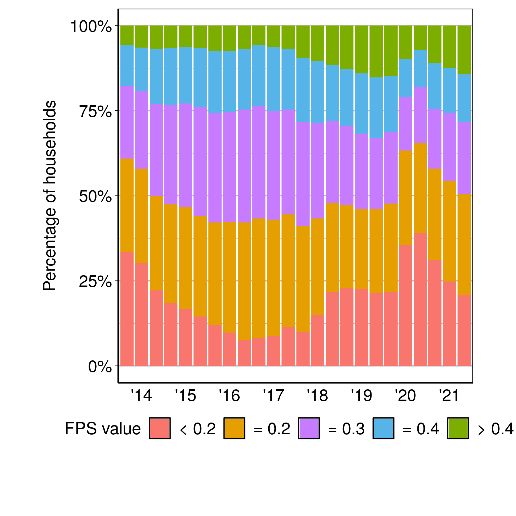
We next examine the cross-sectional variation in household participation. For this, we categorise all households into five groups: those with (1) FPS less than 0.2, (2) equal to 0.2, (3) equal to 0.3, (4) equal to 0.4, and (5) greater than 0.4. Figure 1 shows the fraction of households in each of these FPS categories, in each wave.

Figure 1: Distribution of households by categories of FPS

Figure 1 shows that there was an increase in household financial participation in the early part of this sample, from 2014 up until the end of 2017. (The areas under the sum of FPS categories >= 2 have dropped in this period.) In 2018 and 2019, there was no change in the fraction of households across the defined categories. The changes of 2014-2016 appear to reverse from the second half of 2020 onwards. By 2021, the fraction of households with FPS >= 0.3 is nearly the same as the values seen in 2019.

What was happening at the level of the individual instruments?

In Figure 2, we go below the aggregate FPS into portfolio of individual instruments, including bank accounts, fixed deposits, pensions, post office savings, health insurance, life insurance, mutual funds and listed shares. (We do not include the household holdings of KVP and NSC because these fractions were very small compared to the selected eight instruments in the figure.)

Figure 2: Distribution of households portfolio of individual financial instruments by wave (log scale)

Health insurance had the highest growth (10 percent of households holding to 40 percent of households holding in the sample in a wave). At the same time, life insurance saw a drop (from 60 percent of households holding to 40 percent of households in the sample holding this in a wave). Post office savings saw an increase (from 8.5 percent of household holding to nearly 20 percent of households holding) while pensions saw a decrease (from 25 percent of household holding to around 18 percent). While the numerical values are small, there was strong growth in mutual funds and listed shares.

How different is financial inclusion for rural vs. urban households?

How does the financial participation of urban households compare to rural households? In the following Figure 3, we examine the distribution of rural and urban households in the four FPS categories presented in Figure 1.

Figure 3: Distribution of rural and urban households by categories of FPS

The figures show that the distribution of rural households tend to have lower financial inclusion compared to the urban households. More interesting is the difference in the evolution of financial inclusion between these two groups. Both rural and urban households saw increasing financial participation in 2015 and 2016 compared to 2014. However, financial participation of rural households stalled at the end of 2016, while urban households contend to grow their financial participation. Financial participation for both rural and urban households worsened first in 2018, and then more sharply in 2020, at the time of the pandemic.

We also examine what are the differences in financial instruments holdings behind the variation that we see in the financial participation of rural and urban households. From Figure 4, we can see that rural and urban households are similar in their holding of bank accounts, fixed deposits and post office savings. But they are distinctly different in their holding of EPF, mutual funds and listed shares, where there is a higher fraction of urban households holding these instruments compared to rural households.

Figure 4: Distribution of rural and urban households' portfolio of individual financial instruments

Figure 4 also shows us that the growth in fraction of households holding individual instruments vary between rural and urban households. There was a higher growth in fraction of rural households holding health insurance (from 5 to 40 percent), while for urban households this was lower (from 10 percent to 40 percent). There was a drop in the fraction of rural households holding life insurance compared to no change in the fraction of urban households holding these.

This tells us two pertinent aspects of the growth of financial participation across rural and urban households: first, financial participation by rural households appear more vulnerable to external shocks -- such as demonetisation, the ILFS-NBFC crisis and the pandemic -- than urban households. Second, there is some variation in what types of instruments rural households tend to hold compared with urban households.

In the CPHS sampling strategy, there is a roughly two-times over-weighting of urban locations. The simple summary statistics shown in this article (i.e. unweighted estimates) are problematic; for more precise estimates all summary statistics require appropriate weighting. It is hence particularly useful to see the urban and rural values separately, as has been done here.

Conclusions

It is widely believed that improvements in financial inclusion will translate into reductions of consumption volatility and increased odds of improved lives. Greater research is required on measuring the strength of these relationships. In the standard recipe of phenomenological research, we require measurement of a phenomenon, and then it becomes possible to analyse the causes and consequences.

An important missing link in the field of financial inclusion are tools for measurement. In this article, we have shown a first and simplest measure, an input measure, about use of the formal financial system by households. This measure can be computed at the household level, three times a year, in the CMIE CPHS survey database.

In the summary statistics shown here, there have been only small changes in the overall average FPS over the years under examination. The median value for urban households was 0.3 and the median value for rural households was 0.2. We see a visible decline of the FPS in the lockdowns of 2020, and in the post-pandemic economic recovery, the FPS has come back to near pre-pandemic values. These results suggest numerous questions about causes and consequences, which need to be explored in downstream research.

This ability to observe the FPS at the level of a household enables new kinds of academic research, new kinds of feedback loops for policy makers, and definitions and measurement to help ESG investors overcome principal-agent problems between the investor and the fund, and the fund and the portfolio company.

References:

Andersen, S., Campbell, J. Y., Nielsen, K. M., & Ramadorai, T. (2020). Sources of inaction in household finance: Evidence from the Danish mortgage market, American Economic Review, 110(10), 3184-3230.

Badarinza, C., Campbell, J. Y., & Ramadorai, T. (2016). International comparative household finance, Annual Review of Economics, 8, 111-144.

Banerji, R., Bhattacharjea, S., & Wadhwa, W. (2013). The annual status of education report (ASER), Research in Comparative and International Education, 8(3), 387-396.

Beck, T. (2016). Financial Inclusion–Measuring progress and progress in measuring.

Calvet, L. E., Campbell, J. Y., & Sodini, P. (2007). Down or out: Assessing the welfare costs of household investment mistakes, Journal of Political Economy, 115(5), 707-747.

Campbell, J. Y. (2006). Household finance, The Journal of Finance, 61(4), 1553-1604.

El-Zoghbi, M. (2019). Toward a New Impact Narrative for Financial Inclusion, CGAP, 2019.

Gupta, S., & Sharma, M. (2021). A Demand-Side Approach to Measuring Financial Inclusion: Going Beyond Bank Account Ownership, Dvara Research Working Paper Series No. WP-2021-05.

Monsura, M. P. (2020). The importance of financial literacy: Household's income mobility measurement and decomposition approach., The Journal of Asian Finance, Economics and Business, 7(12), 647-655.

Nguyen, T. T. H. (2021). Measuring financial inclusion: a composite FI index for the developing countries , Journal of Economics and Development, Volume 23, Number 1, pp. 77-99, 2021.

Nilekani N (2019). Report of the High Level Committee on Deepening of Digital Payments, Reserve Bank of India.

Rao, K. S. (2018). Financial inclusion in India: Progress and prospects , The Ideas for India blog, 2018.

RBI (2017). Report of the Household Finance Committee on Indian Household Finance, 24 August 2017.

RBI (2020). National Strategy for Financial Inclusion 2019-2024 .

Sarma, M. (2008). Index of financial inclusion Working paper No. 215, ICRIER, New Delhi.

Sarma, M. (2016), Measuring financial inclusion using multidimensional data, World Economics, 1 Ivory Swuare, Plantation Wharf, London, UK, SW11 3UE, vol. 17(1), pages 15-40, January 2016.

International Finance Corporation (IFC) (2011). Financial inclusion data: assessing the landscape and country-level target approaches. The World Bank, 2011.

United Nations Environment Program Finance Initiative (UN EPFI) (2021). 28 Banks collectively accelerate action on universal financial inclusion and health, 2 December 2021

Geetika Palta, Mithila Sarah and Susan Thomas are researchers at the XKDR Forum. We thank Ajay Shah and three anonymous referees for valuable comments and suggestions.

History of disinvestment in India

by Sudipto Banerjee, Renuka Sane, Srishti Sharma and Karthik Suresh.

Disinvestment of public sector enterprises has been an important part of Indian economic policy since the 1990s. Research in this field has been constrained by a lack of foundations of facts. There is limited information on policy positions, policy actions, as well controversies around policy actions. For example, Baijal (2008) provides a history of early disinvestment decisions in India; Banerjee Sane and Sharma (2020) provide information on the more recent methods adopted for disinvestment; Banerjee, Moharir and Sane (2020) document disinvestments undertaken to meet the minimum public shareholding rule in India.

In a new working paper, History of disinvestment in India: 1991-2020, we contribute to the literature by documenting the history of disinvestment of Central Public Sector Enterprises (CPSEs) in India between March 1991 to December 2020. The paper is a collection of facts on:

1. The policy position of governments across the years
2. The policy processes adopted by governments on selection of enterprises for disinvestment
3. The difficulties encountered in various transactions on (i) methods of valuation, (ii) legal disputes challenging the transactions, (iii) adverse audit remarks of the CAG, and (iv) labour unrest.
4. Targets for disinvestment and amounts raised
5. The different methods of disinvestment, especially those used in recent years such as compulsory buybacks, Offer for sale through the stock exchange (OFS-SE), CPSE to CPSE sales, Exchange Traded Funds (ETFs), and public offers.

We found it difficult to achieve this level of clarity on the facts, and hope that this helps many others approach the field with better foundations on facts.

References

Baijal, P. (2008), Disinvestment In India: I Lose and You Gain, Pearson; 1st edition.

Banerjee S., Moharir, S., and Sane R. (2020), The problem of minimum public shareholding in public sector enterprises , The Leap Blog, 18 November 2020.

Banerjee S., Sane R. and Sharma, S. (2020), The five paths of disinvestment in India , The Leap Blog, 7 July 2020.

But clouds got in my way: Bias and bias correction of nighttime lights data in the presence of clouds

by Ayush Patnaik, Ajay Shah, Anshul Tayal, Susan Thomas.

Night lights is an opportunity to measure prosperity, using an eye in the sky, without requiring institutional capacity in economic measurement on the ground. The first wave of research used the DMSP-OLS dataset, which had annual images from 1992 to 2013. An improvement in this field was the launch of Suomi-NPP in 2012 where the pixels are smaller (0.5km x 0.5km), and the frequency shifted from annual to monthly. A substantial economics literature has found innovative applications of this data. When research projects are set in India, most researchers have relied on the district-level dataset that is generously released by the World Bank.

In a new paper, 

• We suggest there is a downward bias in the radiance, that is associated with the presence of clouds. The magnitudes are economically significant, e.g. -28% in July for Bombay.
  
• We propose a bias correction scheme that partly corrects for this bias.
• We have released the source code which implements our improved methods and conventional methods, so they can be used in data construction by applied economists and for methodological research in remote sensing.
  

The problem of bias

As an example, consider the radiance seen at the satellite from the city of Bombay:

The red line is the aggregate radiance from Bombay. It shows peculiar annual dips. The vertical dashed lines mark July months, where the monsoon is strongest (on average). The lower graph is the number of cloud-free pixel-days that make up this aggregate radiance. There is a pattern: odd dips in radiance that are correlated with low values for the number of cloud-free pixel-days.

Is this just the seasonality of income, which happens to be correlated with the seasonality of cloud cover? 

The graph above juxtaposes the seasonal factors of monthly aggregate income in Bombay (the black line) vs. the seasonal factors of monthly aggregate radiance for Bombay (the red line). There is no seasonal dip of income in July as is the case with nighttime lights.

This is just an example, for the city of Bombay. The paper has large scale evidence about the presence of this problem more generally.

We conjecture that for a pixel, in a month with a low number of cloud-free images, even on those few days, there are light clouds which attenuate the signal, thus inducing a downward bias in the observed radiance.

A partial bias-correction scheme

When a pixel has both bright and cloudy months in the data, we are able to estimate the bias and correct for it.

There are pixels which are cloudy all through the year. Here, the bias is unidentified.

Our bias-correction scheme works cautiously, only modifying the data when there is high confidence that there is bias and we are able to estimate the magnitude of the bias. It reduces the bias but does not eliminate it.

As an example, consider Bombay:

As before, the black line has the seasonal factors of aggregate income in Bombay. The red line has the seasonal factors of conventionally cleaned night lights data. The dashed purple line has seasonal factors for the night lights data released by the World Bank. 

The blue dotted line is the new bias-corrected night lights data. These seasonal factors are closer to the black line and an improvement upon the two conventional datasets.

Once again, Bombay is just an example; the paper has large scale evidence which demonstrates these gains. For the aggregate radiance of India:

Here also, the dotted blue line (the seasonality of the new night lights data) is closer to the black line (the seasonality of aggregate income in India), and fares better than the two conventional datasets (the World Bank's release or conventionally cleaned nighttime radiance).

Reproducible research

We have released the data and R code to reproduce all our calculations for Bombay. And, we have released a Julia package using which the new tools can be used for methodological research and applications. This software consumes a pixel-level NASA/NOAA VIIRS dataset and returns a bias-corrected pixel-level dataset which will readily fit into analyses of the existing NASA/NOAA VIIRS data. This is also the first open source package for conventional cleaning.

Distribution of self-reported health in India: The role of income and geography

by Ila Patnaik, Renuka Sane, Ajay Shah and S. V. Subramaniam.

In health research, we study the causes and consequences of health at the individual level. This requires measurement of the health status of individuals. One simple path lies in asking a person: "Are you feeling well today?". This `self-reported health' (SRH) is a measure that is easy to implement, and has limitations in that psychological factors are present. A significant global literature has emerged, which draws on this measure to explore the causes and consequences of health.

The CMIE CPHS is an important new dataset which has longitudinal data for about 170,000 households, measured three times a year. They measure SRH for each individual in each wave. This measurement of SRH, alongside a rich array of household characteristics, makes possible many interesting research projects. In a new paper, Distribution of self-reported health in India: The role of income and geography, we discern some new facts and phenomena about health in India, through this data.

We use data for calendar 2018 and 2019, which works out to 3.5 million observation of a person in a wave. These years were chosen in order to obtain a baseline description of health in India, while avoiding the pandemic of 2020 and the possible impact of demonetisation in 2017.

What do we find? On average, ill health is observed in 3.25% of the records. On average, people in India are unwell for about 12 days a year. There is a U-shaped curve in age, with higher ill health rates for the young and the old.

We get a nice map of the variation of the ill-health rate across the country. This is interesting, in and of itself, as it shows us something about health care requirements. However, some of this variation reflects geographical heterogeneity in income and age structure.

We estimate logit models which explore correlations between standard socio-economic measures and the ill-health rate. The important sources of variation turn out to be age, income and location.

We then focus on an approximately modal person. Model-based predictions for the ill-health probability are constructed for this individual. This yields a map of the predicted ill-health rate --  

 

This shows the variation of ill-health in the 102 `homogeneous regions' (HRs), after controlling for income, age structure and other standard socioeconomic characteristics. It is an interesting and new map. These results do not conform with the standard stereotypes of north vs. south. Epidemiological research is required in understanding what is at work in each of the difficult HRs. Major gains in the health of the people could potentially be obtained by focusing on these hot spots and finding the right public health interventions.

We then ask: are rich people healthier than poor people? As the rich fare better on nutrition, housing quality, knowledge and access to health care, we expect there would be such a correlation. This is indeed the case in the overall aggregate data. However, there is strong geographical variation in this correlation. Ill health and poverty are positively correlated in only half of the country. There are even HRs where the relationship is reverse -- where poor people report better health than the rich. Further, the two maps (the map of ill health of the modal person, and the map of the places where ill health is not positively correlated with income) show different patterns. They are distinct phenomena that invite further exploration.

Inflation got back into the target zone

by Ajay Shah.

On 20 February 2015, MOF and RBI signed the `Monetary Policy Framework Agreement', and the power of monetary policy (i.e. setting the short term rate) got connected to an objective (get y-o-y CPI inflation to 4%, with a permissible range from 2 to 6 per cent). For some time thereafter, it worked rather well.

From late 2019, we have had problems with inflation. In December 2019, the bound was breached, when inflation reached 7.36 per cent. In the 12 months from December 2019 to November 2020, there was only 1 month (March 2020) where the value at 5.84 was within the 2-to-6 range.

There was considerable angst about this. For many people, aggregate demand was clearly adversely affected by social distancing, and the task of monetary policy was to stimulate demand. In this period, headline inflation being above 6 per cent was an irritant. It even proved, to some, that the very concept of inflation targeting was flawed. There was the angst that is often heard in India, about supply constraints that shape inflation.

RBI eased monetary policy using the many instruments that it possesses, including the repo / reverse repo rates where the votes of 3 external members of the MPC also count.

In my research network, we felt comfortable about this stance of monetary policy:

• Our models, which work with seasonally adjusted data, suggested that headline inflation would drop in December. 
• We expected that the easing of supply restrictions that comes with post-pandemic normalisation would help address glitches in the price system.
• Our macroeconomic common sense suggested that at a time of weak aggregate demand, inflationary pressure was going to be low. 
•  In any case, monetary policy acts with a long delay. Headline inflation (a moving average of the point-on-point inflation of the latest 12 months) is a poor guide for anticipating headline inflation about one to two years out.
  

These arguments fed into our writings of this period: 7 Apr, 24 Jul, 24 Aug, 4 Dec, 11 Jan (the day before the December CPI release). 

We now have a data release for December 2020 and headline inflation was reported at 4.59 per cent, which is close to the target of 4 per cent, and well below the upper bound of the target range, of 6 per cent:

Headline inflation, in the inflation targeting period

I am reminded of Ken Rogoff who once said "Those who think inflation is caused by too little pork rather than too much money are wrong" (in the Financial Times, 4 February 2008). It speaks well for the Indian economic policy process, that the Ministry of Finance and RBI stayed the course through this period, and protected the inflation targeting system.