Envisioning the INR as a floating exchange rate

by Rounak Hande, Rajeswari Sengupta and Ajay Shah.

The Question

A central question in macroeconomic policy is the exchange rate regime. In the long-run, India's economic strategy should move to a combination of inflation targeting, floating exchange rate and an open capital account. In more than three decades since the economic reforms of 1991, only one of these milestones has been achieved--RBI today is an inflation targeting central bank. For IT to be fully effective, it must be accompanied by a floating exchange rate. However, we in India are used to the idea that the RBI actively intervenes in the FX market to stabilise the USD/INR rate. It is important to ask, What might a genuine floating exchange rate look like if the RBI did not intervene? In other words, If RBI were to the USD/INR what SEBI is to the Nifty, what would that world look like?

When it comes to government price controls on commodities, e.g. wheat, there is a ready way to visualize what a reformed India would look like: the Indian price of wheat would be the world price of wheat. But what about the exchange rate? If the required reforms took place, and we got to a market determined rupee, what would it be like? In this article, we present a reasonable depiction of what the exchange rate regime would be like, if the RBI did nothing on the currency market. This also helps us understand how much currency volatility Indian firms and households need to prepare for if the RBI were absent from the market.

The period of INR as a float

When we look back into India's history, we find that there was one period when trading by the RBI on the currency market dropped to near zero levels. We treat this as a natural experiment to gain insights into what the INR would look like without government control. Our first task is to establish the start and end dates of that period.

We start with three long time-series graphs: (i) RBI's spot market trading volume in USD, (ii) RBI's spot market trading volume relative to reserve money, and (iii) RBI's open position on the currency forward market.

Figure 1: The long time-series of spot price trading volume by RBI, in billion USD

Figure 2: The long time-series of spot price trading volume by RBI, expressed as per cent of M0.

Figure 3: The long time-series of the RBI's currency forward position, in billion USD.

In all these graphs, we can spot one remarkable period, from June 2009 to October 2011, where an important reform of the exchange rate regime took place, and the RBI stepped out of the currency market. Let's zoom into that period. To obtain greater clarity, we focus on the period from June 2006 to October 2014, adding three years to each side.

Figure 4: Spot price trading volume by RBI, in billion USD (June 2006 to Oct 2014).

Figure 5: Spot price trading volume by RBI, expressed as per cent of M0 (June 2006 to Oct 2014).

Figure 6: RBI's currency forward position, in billion USD (June 2006 to Oct 2014).

In these pictures, we see a middle period -- 28 months from June 2009 to October 2011 -- when currency trading by the RBI was very low. The RBI's trading volume in these months was not always 0. In choosing these endpoints, we set a limit where the RBI's gross monthly trading volume stayed below 1 percent of M0.

Examining the characteristics of this period gives us insights into what a floating exchange rate in India might look like.

Characteristics of the INR as a float

In this section we describe the characteristics of the INR in the period from June 2009 to October 2011. For the sake of comparison, we use the methodology described in Sengupta and Shah (2026) to establish the dates of two other exchange rate regimes. We will now focus on three such regimes:

• The natural experiment of the INR as a float: 1st June 2009 to 31st October 2011.
• The recent period of a tight USD peg : 1st September 2023 to 16th December 2024.
• The present exchange rate regime: 27th December 2024 to 28th August 2026 (latest available data).

For each of these periods, we examine (a) The volatility of the USD/INR rate (b) The parameter estimates obtained from the exchange rate regression (see Google colab notebook associated with Sengupta and Shah (2026)) and (c) Deviations from market efficiency as seen in variance ratios.

Metric	Float (June 2009–Oct 2011)	The USD peg (Sept 2023–Dec 2024)	Current ERR (Dec 2024–Aug 2026)
Volatility:
USD/INR vol (%)	7.40	1.43	4.98
The exchange rate regression:
USD	0.66***	0.89***	0.79***
EUR	0.20**	0.05	0.11
JPY	-0.15**	-0.01	-0.08
GBP	0.04	0.05	0.25
R-sq	0.75	0.98	0.76
RSE	0.77	0.18	0.67
Variance ratio tests:
VR(5), daily	0.99	0.67	0.96
p value	0.82	0.03	0.61
VR(4), weekly	1.07	0.64	0.76
p value	0.93	0.03	0.14

We summarise our findings as:

• In the popular discourse on the INR, a lot of attention is given to the raw USD/INR volatility. At present, it is running at 4.98 percent. During the period of the USD-peg, it had fallen to 1.43 percent. We see that under the float, it was 7.4 percent. In other words, if the RBI did not intervene in the currency markets, the USD/INR volatility that the economy could experience is around 7-7.5 percent. Later in the article, we speculate on how things might work out if the INR were to return to a float under the present conditions and we argue that the volatility could be lower.

  The numbers also suggest that during the current exchange rate regime (27th December 2024 to 28th August 2026), the machinery of the RBI's currency policy seems to have delivered only a small decline in volatility of about 2.4 percentage points on an annualised basis.

• In the exchange rate regression, during the period of the USD peg, the USD coefficient was statistically significant with a value of 0.89, and no other currency was significant. At present, the USD coefficient has come down to 0.79, but still, none of the other currencies have statistically significant coefficients.

  In contrast, during the period of INR float, the USD coefficient was smaller at 0.66, and other currencies were significant too. This suggests that the Indian economic engagement with the outside world is not merely with the US. In the float period, USD, EUR and JPY were all statistically significant, with coefficients of 0.66, 0.2 and -0.15. This gives us an undistorted sense of the currencies that matter for the Indian economy.

• Another important statistic from the exchange rate regression is the residual standard deviation (or RSE, residual standard error). It shows the size of the prediction error of the exchange rate regression. A lower RSE means the model fits the data well. Therefore, during the period of the USD peg, the residual standard deviation was only 0.18. In contrast, under the INR float the RSE was 0.77. In the current regime, the RSE stands at 0.67.

• In the exchange rate regression, during the period of the USD peg, the R-squared was 0.98. A high R-squared value implies that almost all of the variation in the INR was accounted for by the currencies in the regression model. At present, the R-squared has fallen to 0.76. During the INR float, the R-squared had a very similar value, 0.75. In other words, despite active trading by the RBI in the currency market in the present period, there is not much of a difference in the R-squared.

  This yields insights into deciphering a floating exchange rate regime from the data. A floating exchange rate does not necessarily mean an R-squared value close to 0. It means that the central bank does not intervene and lets the exchange rate respond freely to market forces. In a floating regime, the R-squared value can still be high because it reflects the natural, underlying co-movement of the rupee with major currencies of the world (and not just the USD) under conditions of globalisation. India is deeply interconnected with these countries through trade and financial flows, and is exposed to the same global shocks. Some co-movement is therefore entirely consistent with a genuine float.

• The variance ratio test is a simple tool to examine serial correlations. A floating exchange rate is expected to be an efficient market, with no discernible serial correlation, and no exploitable profit opportunities for trading based on time-series characteristics. This does work out correctly in the float period. In the daily data, the 5-period variance ratio was 0.99, and indistinguishable from 1, whereas in the weekly data, the 4-period variance ratio was 1.07 and indistinguishable from 1. Under the USD peg, the two variance ratios were 0.67 and 0.64, with statistically significant deviations from non-forecastability. In the present arrangement, the variance ratio at 4 weeks is away from 1.

A useful variant of the exchange rate regression, introduced in Kumar et. al. (2020), differentiates between the USD coefficient when faced with a USD appreciation vs. a depreciation thereby highlighting asymmetric intervention by the RBI. We now turn to these estimates.

Metric	Float (June 2009–Oct 2011)	The USD peg (Sept 2023–Dec 2024)	Current (Dec 2024–Aug 2026)
USD (App)	0.52***	0.87***	0.68***
USD (Dep)	0.83***	0.91***	0.88***
EUR	0.20***	0.05	0.12
JPY	-0.15***	-0.01	-0.09
GBP	0.04	0.05	0.24
R-sq	0.77	0.98	0.77
RSE	0.74	0.18	0.66

During the period of the USD peg, it is not surprising to see statistically significant values of the USD coefficient close to 1, for both USD appreciation and USD depreciation. This makes sense because when the RBI is pegging the INR to the USD, it is expected that currency interventions would take place on both sides of the market, regardless of which way the USD is moving. In the present exchange rate regime, the INR responds more strongly to a USD depreciation (with a coefficient of 0.88) than it does to a USD appreciation (with a coefficient of 0.68). This implies that the RBI now intervenes asymmetrically, letting the INR move more freely when the USD appreciates (i.e. the INR depreciates) but managing the INR more when the USD depreciates (i.e. the INR appreciates). This is consistent with existing studies documenting the RBI's asymmetric intervention patterns (Patnaik and Sengupta, 2022). RBI prefers buying dollars (preventing INR appreciation) over losing reserves (preventing INR depreciation).

Interestingly however, we find asymmetric coefficients in the floating period too, with a response of 0.83 when the USD depreciates but a coefficient of 0.52 when it appreciates. This is puzzling because in a float, there should be no asymmetry between these coefficients, both of which should be equally low. Further research is therefore required to understand the market-based sources of this asymmetry.

Conclusion

In the strategic view of macroeconomic policy, the long-run answer for India lies in graduating from one milestone -- inflation targeting -- to two more milestones -- a floating exchange rate and an open capital account.

At every stage in the journey of Indian economic reforms, the prospect of getting the government out of price determination has raised alarms in the minds of some people. When the proposals to remove price controls for steel or cement were made, there was shock and unhappiness in the minds of many people. These things are often easier done than said, because the price system works rather well. It solves the resource allocation problem, and prices move continuously in a way that provides good incentives to private persons.

In this article we have shown one tangible period, of 883 days, in which the RBI stayed away from the currency market and there was a genuine floating exchange rate. This period can be utilised for many other research projects. Using the insights from this period, we are now able to offer a thumb rule to judge the extent of government management of the exchange rate in India in terms of three numbers. For example, we can compare the values observed today of (i) the USD/INR volatility of 4.98 percent, (ii) the USD coefficient of 0.79, and (iii) the RSE of 0.67 vs. the values observed during the float: (i) the USD/INR volatility of 7.4 percent, (ii) the USD coefficient of 0.66, and (iii) the RSE of 0.77. This gives us a sense of how much government control of the exchange rate is present today.

This natural experiment, of a country that graduated to a floating exchange rate and then retreated from it, gives us insights on how to interpret the estimates from the exchange rate regression and the toolchain of Zeileis et. al (2010).

Looking into the future, when economic policy reforms take place in India, we believe the USD/INR volatility under a true floating exchange rate will be lower than this value of 7.4 percent, for two reasons:

1. There is one important difference between the float period of 2009-2011 and the future: Inflation Targeting. That RBI movement to a floating exchange rate was incomplete because it was not accompanied by inflation targeting. In some sense, that was a particularly unfortunate event as the rupee lost its nominal anchor during that period. In the future, things will be better because now the nominal anchor is 4 percent CPI inflation.
2. Another important difference concerns the liquidity of the USD/INR spot and derivatives markets. In the 2009-2011 period of INR float, these markets were less developed. We estimate that in that period, the total turnover(onshore and offshore) was about USD 40 billion per day. By now, things have improved, with a huge increase in INR activity outside India. Now the total turnover (onshore and offshore) is about USD 140 billion per day. This bigger market delivers greater stability. Hence, we can speculate that in the future, things will be better in terms of USD/INR volatility.

References

Kumar, S H, Balasubramaniam, V, Patnaik, I and Shah, A (2020), "Who cares about the Renminbi?", Working Paper, December 2020.

Patnaik, Ila and Rajeswari Sengupta (2022) "Analyzing India's Exchange Rate Regime", India Policy Forum, National Council of Applied Economic Research, vol. 18(1), pages 53-85.

Sengupta, R and Shah, A (2026), "Words and deeds in the Indian exchange rate", The Leap Blog, May 19, 2026.

Zeileis, A, Shah A, and Patnaik, I (2010) "Testing, monitoring, and dating structural changes in exchange rate regimes", Computational Statistics & Data Analysis, Volume 54, Issue 6.

Rounak Hande and Ajay Shah are researchers at XKDR Forum, Mumbai and Rajeswari Sengupta is a researcher at IGIDR, Mumbai.

Words and deeds in the Indian exchange rate

by Rajeswari Sengupta and Ajay Shah.

The most important price in any economy is the exchange rate. In India's case, this is the price of the Indian rupee against the US dollar. By default, the exchange rate is controlled by market forces. The policy stance of the government, towards the exchange rate, is termed 'the exchange rate regime'. This is one of the most consequential economic policy choices.

In most advanced economies, the answer is straightforward: the exchange rate is set by financial markets, and the government stays out. In India, it is more complicated. The RBI regularly intervenes in the foreign exchange market. India's exchange rate regime needs to be deciphered from the data using statistical tools.

At any point in time, to understand the Indian economy, knowing the present exchange rate regime is central. Looking back at economic history, knowing the dates and characteristics of the changing exchange rate regime is central.

Inferring the true exchange rate regime from the data

We now have mature tools for deciphering the exchange rate regime using exchange rate data, without requiring information about the actions taken by the government. This runs in two steps: the first is a sweet linear regression called 'the exchange rate regression' and the second is the econometrics of structural change through which structural breaks in the regression coefficients and the residual standard deviation are detected. This idea for structural breaks in linear regression models where the residual standard deviation can also change is taken from Zeileis, Shah and Patnaik (2010) and implemented in the R package fxregime which now has numerous applications into fields well beyond exchange rate regimes and structural change.

In this article we will first rev up this tool chain for the Indian rupee, offering measures of the present exchange rate regime and of the history of Indian macroeconomic policy. We will then turn to a comparison against RBI and IMF statements about the Indian exchange rate regime. Finally, we will offer ready access to reproducible research so that everyone can perform these calculations.

Reading the data: six distinct regimes since 2000

The exchange rate regression estimates how much of the movement in the rupee is explained by movements in the world's major floating currencies - the US dollar, the euro, the British pound, and the Japanese yen. The greater the role of these foreign currencies in explaining the rupee's movement, the less independently the rupee is floating. Alongside this, we get the residual standard deviation: the extent to which the movements of the rupee reflect none of the above. The dates of structural breaks mark the boundaries between different exchange rate regimes.

We apply this method to weekly exchange rate data from the BIS, covering the period from 1 January, 2000 to the most recent data available at the time of publication (15 May, 2026). The analysis shows six distinct exchange rate regimes. This gives us an updated version of the knowledge in Patnaik and Sengupta (2022) and Pandey, Patnaik and Sengupta (2024).

Figure 1: USD/INR exchange rate with structural breaks.

Figure 2: Annualised volatility of USD/INR (6 month rolling window) with structural breaks.

The six periods are as follows:

Regime 1 (14 January 2000 - 19 March 2004): This was a tight peg to the dollar. The rupee moved very little independently. The annualised INR-USD volatility averaged just 2.2%.

Regime 2 (26 March 2004 - 16 March 2007): This was a move towards greater flexibility. The rupee was moderately pegged to a basket of currencies. The volatility rose to 4.1%.

Regime 3 (23 March 2007 - 13 December 2013): This was the most flexible period in the 25 years under examination. This was the era when India came closest to a genuinely market-determined exchange rate. The USD/INR volatility was 8.7%. There were many months in this period where RBI trading on the currency market was 0. This gives us an interesting conjecture: If the rupee were to float, it would have an annualised vol of about 9%.

Regime 4 (20 December 2013 - 25 August 2023): This was a retreat to greater currency management. This was the longest single regime in our sample - nearly a decade. The INR-USD volatility fell back to 5%, and the RBI's interventions in the foreign exchange market grew steadily. It is ironic that inflation targeting came into India in February 2015, with the signing of the Monetary Policy Framework Agreement. This was roughly the same time that rupee flexibility was in retreat.

Regime 5 (1 September 2023 - 20 December 2024): A remarkable de-facto peg; the lowest volatility in 25 years. For this 15-month period, INR-USD volatility was just 1.5%: the lowest in our 25-year sample, lower even than Regime 1 which reflected the macroeconomics knowledge of long ago. The rupee barely moved against the dollar, even as other emerging market currencies fluctuated.

Regime 6 (27 December 2024 - 15 May 2026): Finally, we got a partial retreat from the peg. Volatility rose to 5%, comparable to Regime 4. In our analysis, this regime ends on 15 May 2026, because that is the latest available data.

What the RBI says

In 1993, India officially moved towards a "market-determined exchange rate". The RBI website states that its "exchange rate policy focuses on ensuring orderly conditions in the foreign exchange market" - implying that it intervenes only to prevent excessive volatility, not to target any particular level of the rupee.

The empirical evidence, however, shows that the Indian economy experienced six different exchange rate regimes without any changes in official statements, announcements, or rationale.

What the IMF says

The International Monetary Fund, which classifies every member country's exchange rate regime every year, had long described India's regime as "floating", noting that the rupee is "largely market determined" and that the RBI intervenes only to manage "excessive volatility". The IMF classification does not see the six regimes that the data reports.

Figure 3: USD/INR exchange rate with regime classification from IMF AREAER.

The econometrics of structural change shows the recent nearly-fixed exchange rate regime as running from 1 September 2023 - 20 December 2024. This event was so large and remarkable that the IMF picked it up. In its 2023 Annual Report on Exchange Arrangements and Exchange Restrictions (released in December 2024), the IMF reclassified India's de-facto exchange rate regime retroactively:

"Since December 2022, the exchange rate stabilized within a 2% band against the US dollar, with one realignment in August 2023. Therefore, the de facto exchange rate arrangement was reclassified retroactively to 'stabilized' from 'floating', effective December 6, 2022."

The structural change econometrics picks up different dates compared with these statements. The statistical techniques isolate precise dates for structural breaks down to the week, in contrast to the IMF classification, which is updated annually.

The centrality of the exchange rate regime in the Impossible Trinity

The Impossible Trinity is a foundational concept in economics. It states that a country can achieve at most two of the following three objectives simultaneously: an open capital account (allowing money to flow freely in and out of the country), a fixed or managed exchange rate, and an independent monetary policy. It is impossible to have all three at once.

India adopted inflation targeting in February 2015, which means it chose to have autonomy in domestic monetary policy with the legal mandate to keep CPI inflation at 4%. India also has a substantially open capital account after three decades of gradual liberalisation. According to the Trilemma, these two choices leave no room for a managed exchange rate. India cannot simultaneously target 4% inflation, maintain an open capital account, and stabilise the rupee against the dollar.

Yet the data show that from late 2022 to late 2024, that is what the RBI attempted to do. In this period, India's nominal anchor - what the monetary system was supposed to be anchored to - quietly shifted from the inflation target to the exchange rate. In effect, RBI's legal mandate under IT was temporarily displaced by an unannounced exchange rate objective. These attempts induce many difficulties; financial restrictions impeded economic growth, and inflation was excessively volatile owing to the pursuit of extraneous objectives.

Macroeconomic stability requires credibility of monetary policy. Under inflation targeting, the authorities must say what they will do, and then do what they just said. Even if all the right things are done immediately, it would take decades for private persons to learn to trust that there is a stable framework of macroeconomic policy.

It is easy to do these calculations

We have made this analysis a self-contained Google Colab notebook, which can be used by you to do runs or classroom teaching.

References

Radhika Pandey, Ila Patnaik and Rajeswari Sengupta (2024) "The journey of inflation targeting in India," Indira Gandhi Institute of Development Research, Mumbai Working Papers 2024-022, Indira Gandhi Institute of Development Research, Mumbai, India.

Patnaik, Ila and Rajeswari Sengupta (2022) "Analyzing India's Exchange Rate Regime," India Policy Forum, National Council of Applied Economic Research, vol. 18(1), pages 53-85.

Zeileis, Achim, Ajay Shah and Ila Patnaik (2010) "Testing, monitoring, and dating structural changes in exchange rate regimes", Computational Statistics & Data Analysis, Volume 54, Issue 6.

The authors are researchers at IGIDR, Bombay and XKDR Forum, Bombay, respectively. The authors thank Rounak Hande for excellent research assistance with the data and analysis, and Anjali Sharma for valuable discussions and comments.

Reinforcing the Anchor: The Next Five Years of Inflation Targeting in India

by Rajeswari Sengupta and Ajay Shah.

The adoption of inflation targeting (IT) in 2015 marked a watershed in India's monetary policy. It is a delight to look back to those dramatic weeks. For the first time since its establishment in 1934, the Reserve Bank of India (RBI) graduated from being a `temporary provision', to a clear legal mandate to maintain consumer price index (CPI) inflation at 4 percent. This shift to a rule-based and transparent framework, with price stability as the explicit objective, strengthened the RBI's credibility, and helped anchor household inflation expectations by reducing the importance of extraneous objectives.

After the Monetary Policy Framework Agreement, the statutory basis for IT was provided by the Reserve Bank of India Amendment Act (2016). In this, the government, in consultation with the RBI, must review the inflation target every five years. The precise text of this section is:

45ZA. Inflation target - (1) The Central Government shall, in consultation with the Bank, determine the inflation target in terms of the Consumer Price Index, once in every five years.

The next review is scheduled for March 2026. In preparation for this process that would be led by the government, the RBI has released a discussion paper seeking public feedback on four specific questions:

1. Whether headline inflation or core inflation would best guide the conduct of monetary policy, given evolving relative dynamics of food and core inflation and the continuing high weight of food in the CPI basket?
2. Whether the 4 per cent inflation target continues to remain optimal for balancing growth with stability in a fast growing, large emerging economy like India?
3. Should the tolerance band around the target be revised in any way including whether the tolerance band be narrowed or widened or fully done away with?
4. Should the target inflation level be removed, and only a range be maintained within the overall ambit of maintaining flexibility without undermining credibility?

Targeting headline vs. core inflation

A substantial body of academic research and cross-country evidence informs the debate on whether central banks should target headline or core (excluding food and energy) inflation (Pandey and Patnaik, 2020). Walsh (2011) shows that in low-income economies, food inflation is more persistent than non-food inflation, with shocks to food prices spilling over into non-food prices. In such contexts, an exclusive focus on core inflation risks mis-specification. Empirical studies further document sizeable second-round effects from headline to core inflation, driven by the high share of food in household expenditure and the role of food inflation in shaping expectations and wage-setting (Anand, Ding, and Tulin, 2014).

The core function of monetary policy in this context is not to control the first-round effects of a supply shock (e.g., a poor monsoon), but to prevent them from propagating into generalised inflation through second-round effects on wages and expectations. This would be best achieved by having a credible central bank that fully devotes all the power of monetary policy to the pursuit of one transparent objective, headline inflation.

The Indian case illustrates these dynamics clearly. Food and fuel account for half of the household consumption basket, so excluding these components would eliminate a large share of relevant prices from the inflation measure. The Urjit Patel Committee Report (RBI, 2014) underscored that elevated food and energy inflation typically translates into higher inflation expectations, with lagged effects visible in services and other components. Moreover, shocks to food and fuel prices have larger and more persistent effects on inflation expectations than shocks to non-food, non-fuel items. Since anchoring expectations is central to the success of inflation targeting, a framework that sidelines food and fuel inflation would be incomplete.

The cross-country evidence reinforces this conclusion. As documented by Pandey and Patnaik (2020), most inflation-targeting economies use headline inflation as their target. A few, such as Thailand, initially targeted core inflation but later shifted to headline inflation in recognition of its greater relevance for households and firms.

Headline inflation has further advantages. It reflects the cost of living most relevant to households, shaping both their consumption and investment decisions (including choices between financial assets, gold, and real estate). It also serves as the benchmark for firms' price-setting behavior. Since monetary policy ultimately seeks to anchor public expectations, and central bank accountability operates through the political system, credibility depends on targeting the measure most salient to the public.

For these reasons, despite the argument that much of CPI inflation lies outside the direct influence of monetary policy, excluding food and energy would not yield a meaningful measure of inflation for policy purposes. While monetary policy cannot influence a poor monsoon, it is the only tool capable of preventing the resulting food price shock from de-anchoring inflation expectations and triggering a wage-price spiral. Targeting headline inflation forces the Monetary Policy Committee to remain vigilant against these second-round effects, which is the essence of a credible IT framework. Therefore, headline inflation remains the most feasible and appropriate target for the conduct of monetary policy in India.

The 4 percent inflation target

The inflation target should remain at 4 percent. Raising it would risk eroding public confidence in the RBI's ability to control inflation, un-anchoring expectations and undermining the credibility of the framework. From a public debt management point of view, an unanticipated increase in the inflation target is tantamount to a partial debt default. Indeed, higher targets and wider bands are associated with greater output and inflation volatility (Horvath and Mateju, 2011).

Conversely, a reduction to 2 percent would only be feasible once India's financial system is sufficiently developed to operate with limited policy space near the zero lower bound - a condition still many decades away. The sequencing there lies in first getting up to FSLRC level financial economic policy, having it stabilise for about a decade, and then examining the possibility of going down to a 2% target. This is perhaps 25 years away.

Tolerance band around the 4 percent target

The literature broadly agrees that price stability corresponds to an inflation of 1-3 percent in advanced economies, while for emerging economies the relevant range is 4-5 percent (RBI, 2014). Empirical estimates for India place the growth-impeding threshold of CPI inflation at 6 percent. Accordingly, the 1-3 percent benchmark for advanced economies provides a lower bound, while 6 percent marks an upper bound for India. As explained in the Urjit Patel Committee Report, this rationale underpinned the adoption of a 2-6 percent tolerance band under India's inflation-targeting regime.

The principal merit of a band is that it allows a central bank that possesses a weak monetary policy transmission to have failures on meeting the inflation target without a loss of credibility. Back in the 2013-2015 period, there was a `learn to walk before you can run' reasoning around this: it was a fully new idea, that RBI should target inflation, so it was better to start with an easier objective.

Having operated within this framework for a decade, the RBI has established a minimally viable inflation-targeting regime. The logical next step would now be to narrow the band to 3-5 percent, which would strengthen credibility and inspire greater public confidence than the relatively wide 2-6 percent range. Critics may argue that a narrower band increases the risk of a technical breach, potentially harming the RBI's credibility. However, after nearly a decade of experience, the institution should possess the maturity to manage this tighter constraint and, if a breach occurs, to communicate its causes effectively to the public. The credibility gains from signaling a stronger, more precise commitment to the 4 percent target outweigh the communication challenges of a potential supply-shock-driven breach. It shows progress; it signals a move from a nascent to a mature IT regime; it enhances respect for India's continued progress towards better institutions.

Range vs. Point target

Point targets with tolerance bands provide clarity and precision, while their symmetry conveys that the central bank seeks to avoid both deflation and inflation (Hammond, 2012). By contrast, pure range targets risk signaling weaker control over inflation. Consistent with this, most inflation-targeting countries adopt a point target with a tolerance band (Pandey and Patnaik, 2020). For households, moreover, a single, well-communicated number aids planning and decision-making, reinforcing the value of a widely recognized 4 percent target. When wage raises are being planned, we need for decision makers to not look at current and future inflation, but instead think that a 4% nominal wage hike is a 0% real wage hike.

Conclusion

Since its adoption in 2016, inflation targeting has enhanced the RBI's monetary policy credibility (Garga, Lakdawala and Sengupta, 2024). Since its adoption, the IT framework has been a crucial institutional anchor for India's macroeconomic stability. The forthcoming review is an opportunity not to question its fundamental design, but to reinforce it. Maintaining the 4 percent headline target while narrowing the tolerance band to ±1% would signal a confident evolution towards a more mature and credible monetary policy, safeguarding the hard-won gains in anchoring public expectations.

References

Anand, Rahul, Ding Ding, and Volodymyr Tulin (2014) Food Inflation in India: The Role for Monetary Policy, IMF Working Papers 14/178; International Monetary Fund.

Garga, Vaishali, Aeimit Lakdawala and Rajeswari Sengupta (2024) Assessing Central Bank Commitment to Inflation Targeting in Emerging Economies: Evidence From India,Working Papers 107, Wake Forest University, Economics Department.

Hammond, Gill (2012) State of the art of inflation targeting,Handbooks 29; Centre for Central Banking Studies, Bank of England.

Horvath, Roman and Jakub Mateju (2011) How Are Inflation Targets Set?In: International Finance 14.2, pp. 265-300.

Pandey, Radhika and Ila Patnaik (2020) Moving to Inflation Targeting NIPFP Working paper 316, August 2020.

Walsh, James P (2011) Reconsidering the Role of Food Prices in InflationIMF Working Papers 11/71; International Monetary Fund.

The authors are researchers at IGIDR, Bombay and XKDR Forum, Bombay, respectively.

How "Orderly" is the Evolution of the Indian Yield Curve?

by Harsh Vardhan.

"Financial market stability and the orderly evolution of the yield curve are public goods and both market participants and the RBI have a shared responsibility in this regard."

Shaktikanta Das, Governor, RBI, October 2020

"Right from October 2020, we have given explicit guidance to the bond market. We expect an orderly evolution of the yield curve, it cannot be otherwise,"

Shaktikanta Das, Governor, RBI, February 2021

As the Covid pandemic has ebbed, central banks across the world are withdrawing the extra-ordinary easy monetary policy that was followed by them since the onset of the pandemic. Reserve Bank in India (RBI) is no exception. A week ago, it took the extra ordinary step of convening an ad-hoc meeting of the monetary policy committee (MOC) to hike the policy interest rates by 40 basis points and also increase the cash reserve ratio (CRR) for banks to take out liquidity from the banking system.

As this “normalisation” of the monetary policy unfolds, its impact on the financial stability has become a matter of concern. The statements of the RBI Governor quoted above, reflect the concern RBI has on financial stability and the evolution of the yield curve. While financial stability is a broad, all encompassing term, evolution of the yield curve is a much more specific idea that can potentially be objectively assessed. In this article I try to assess the orderliness of the evolution of the yield curve over the last four years.

Yield curve describes the basis interest structure in the economy. As the central bank takes policy actions bonds markets reprice the yields and the shape of the yield curve changes. As a fundamental input to pricing of a wide array of assets, predictable and orderly evolution of the yield curve is indeed desirable. High volatility and unpredictability in the evolution of the yield curve, especially when the policy actions taken to normalise monetary policy and regain the GDP growth trajectory post the pandemic, could result in mispricing of financial assets. RBIs concerns and expectation of such orderly evolution are understandable.

In this article, I try to assess the orderliness of evolution of the yield curve. I use data on the yield curve for the 4-year period of 1 April 2018 to 10 May 2022 to empirically assess how the yield curve has changed during this period. To be clear, this article does not evaluate the merits of the RBI’s intent or efforts at managing the yield curve; it only attempts to empirically assess how the yield curve has behaved over this period.

Assessing the evolution of the yield curve:

While it is easy to understand why policy makers would want the yield to evolve in an “orderly” manner in response to policy actions, it is not very easy to define what exactly an orderly evolution means. Trading in government securities takes place every day where all types of financial institutions participate. Even the RBI, through its treasury operations and open market operations participates in the government bond market. The collective actions of all these players determine the prices of government bonds and hence the yield on them.

We could hypothesise orderly evolution to mean that the daily changes in the yields across the curve are smooth and stable. There are two parameters we can look at the describe such smooth and orderly evolution – the volatility of daily yield change and the correlation of changes in yields across varying maturities. If the volatility of daily change in yields remains low and the correlation of yield changes across maturities is high, then it would mean that the yield curve is moving with the policy rates, in a non-disruptive and predictable manner. Such a yield curve can be considered as evolving orderly. On the other hand, increased volatility of daily change and reduced correlation would signal increase in the “disorder” in the evolution of the yield curve.

Data and analysis:

The data for this analysis is the daily yields data on the 3 month treasury bills (T Bills), 1 year, 3, year, 5 year, and 10 year maturity government securities (GoI securities) from 01 April 2018 to 10 May 2022, a total of 993 trading days of data obtained from Bloomberg. Of these maturities the 10-year securities are the most liquid and provide data for every trading day. For the other securities there are days where there would be no trading and hence no data would be available. We consider the previous days yield to continue for such non trading days which means that the change in yields for such days is considered to be zero.

For the purpose of my analysis, I divide the data into 4 time periods as follows:

The first period is from 1 April 2018 to 11 February 2019 which can be called the "pre low interest rate" period. RBI started cutting policy rates from February 19 up until May of 2020. Hence this is the period of stable policy rates. This period has data for 215 trading days.

The second period is from 19 February 2019 to 31 October 2020 is the "downward policy rates and pandemic period" when policy rates were reduced regularly to hit the lowest rate of 4% of repo by May 2020. I extend the period to Oct 31,2020 as RBI clearly started focusing on orderly evolution from October onwards. This period gives us data on 411 trading days.

The third period is from 01 November 2020 to 31 December 2021 which starts with the date of RBI publicly announced its focus on orderly evolution of the yield curve and ends with roughly the end of the pandemic and the reopening of the economy. While the end date is admittedly somewhat arbitrary it coincides with global trend towards rising rates that started in January 2022. This period gives us data on 282 trading days.

The fourth and the shorted period is from 01 January 2022 to 10 May 2022 is the last period where Indian interest rates started inching up (along with interest rates across the world). It includes a few days of data post the surprise, out of turn policy rate hike in May 2022. This period has data on 85 trading days.

For each of these four periods, I compute the following:

• Daily change in the yields of each of the four maturity GoI securities.
• Average daily yield change and the standard deviation of the change in the daily yield which I use as the measure of volatility of the daily change.
• Correlation between yield changes of these 4 GoI securities.

Results:

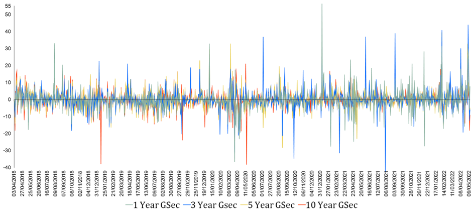
Figure 1 below presents a chart of the daily yield change in these 4 securities over this entire period of little over 4 years and 993 trading days.

Figure 1: Daily Change in Yields on GoI Securities in Basis Points

Source: Bloomberg, author’s analysis

Overall, the chart shows that the volatility of the daily change seems to go up with the onset of Covid in March 2020 with larger and more frequent spikes. This is especially true for the lower maturity; the 3 year and the 1 year maturity securities.

In order to understand the trends in the pattern of the daily change in yield, I plot the 30-day moving average of the daily change in yield as presented in Figure 2 below.

Figure 2: 30 Day Moving Average of Daily Change in Yields on GoI Securities in Basis Points

Source: Bloomberg, author’s analysis

Figure 2 clearly shows a pattern in the changes in the yield curve. The first period has much smaller change daily change in the curve and the changes across maturities are fairly highly correlated. The second period shows much more volatility in the daily change and a significant reduction in the correlation between yield change across maturity. This volatility comes down in the third period and the correlation improves, probably as an outcome of RBIs repeated exhortations and possibly actions in the bond market. The last period shows further reduction in volatility but the correlation is still lower than in the first period indicating that RBIs notices to the bond market and actions have had some success.

In order to more concretely understand the volatility and correlations across these periods, next two charts present the mean daily change in yields and the volatility of the daily change measured as the standard deviation of the daily change in yield.

Figure 3: Mean Daily Change in Yields on GoI Securities

Source: Bloomberg, author’s analysis

This chart clearly describes the interest rate trends in these four periods. The first period had, by and large, stable yield curve with very small changes in yields. The second period shows a secular decline in interest rates across all maturities in response to policy rate changes. The third period shows a reversal of trends and modest rise of interest rates ie the upward movement of the yield curve which becomes much more pronounced and sharper in the fourth period.

Figure 4: Volatility of Daily Change in Yields on GoI Securities

Source: Bloomberg, author’s analysis

This chart shows that the volatility of yield changes has indeed gone up noticeably in the third period when the overall rates showed an increase. The volatility increased especially for the shorter maturity papers – 1 year and 3-year maturity. This probably is the basis of the RBIs focus on ‘orderly’ evolution and hints to the bond market of its discomfort with high volatility. The fourth period shows that the elevated volatility has persisted which means that the bond market has responded only modestly to the RBI’s exhortations. Another important feature to note is that the volatility of the 10 year and the 5 year maturity securities has been contained in the third and the fourth period while that of the shorter maturity securities has continued to remain high. This possibly could also be due to RBI’s targeted interventionsh in the bond market to contain the rise and volatility of yields on long term securities.

Finally, I look at the correlations of yield changes across these maturities. Table below presents the correlation matrix of the four periods.

Table: Correlation Matrix for Yield Change in GoI Securities of Varying Maturities

Source: Bloomberg, author’s analysis

The correlation matrix shows high correlations between yield changes in the first period that start going down in the second period and decline precipitously in the third period. While they improve in the fourth period, they are still below the high levels of the first period. Clearly, the yield curve moved more haphazardly in the third period with high volatility and low correlation between yield changes across maturities. The fourth period shows improvement in correlations probably due to RBIs constant notices to the bond market (and its possible interventions in the market), they do not reach the levels of the first halcyon period.

Conclusion:

This data shows that RBI concern on orderly evolution of yield curve is well placed. The data clearly shows that in period 2, as the policy rates came down, the yield curve volatility shot up. It may well be that the RBI’s focus during this time was on keeping the long-term interest rates low to facilitate economic recovery during the pandemic. The bond market, on the other hand, was concerned about the economic impact of the pandemic and resulting tussle between the RBI and bond market participants actions resulted in increased volatility and break down of correlations in yield movements across maturity. RBI became aware of this volatility towards the third quarter of fiscal 2022 and realised that low rates will not be enough for economic recovery and the excess volatility must be curbed. As it started expressing its desire of an orderly evolution (accompanied possibly by market interventions) there was a modest decline in volatility and improvement in correlations. However, the markets are still not anywhere close to the halcyon pre-pandemic period.

Harsh Vardhan is an independent management consultant and researcher based in Mumbai. The author thanks Surbhi Bhatia for research assistance, and Josh Felman and anonymous referees for very useful comments

Sudden Rise of the Floaters

by Rajeswari Sengupta and Harsh Vardhan.

The first two months of 2021-22 have witnessed a remarkable new trend in the corporate bond market—a sudden rise in the issuance of floating rate bonds or “floaters” and the use of the 91-day treasury bill yield as the reference rate in these bonds, instead of the yields on dated government securities (G-Secs).

We conjecture that one possible reason behind this new development could be an increase in the perception of interest risk on the part of the bond market participants. This in turn may have been a result of the active yield curve management undertaken by the Reserve Bank of India (RBI). If indeed dated government bonds such as the 10-year G-Secs have lost relevance as benchmark securities then this can lead to serious mispricing of risk in the economy, an unintended consequence of the RBI’s bond market intervention.

An interesting development in the bond market

Over the three-month period from April to June 2021, about 7 percent of the total corporate bond issuance of Rs 1.02 trillion consisted of floating rate bonds. While this percentage looks small, it is important to keep in mind that for the previous ten years or more, the share of floating rate bonds in the total issuance of corporate bonds has been less than 1 percent.

It is also important to note that the firms issuing these bonds and the investors investing in them are not a new class of issuers and investors. They are the same issuers and investors who were issuing and buying fixed-rate bonds until recently. In particular, 100 percent of the floating rate bond issuers now are non-banking finance companies (NBFCs) who were earlier issuing fixed rate bonds, and the investors are the same mutual funds and banks who were investing in fixed rate bonds earlier. This could imply that their behaviour has now changed due to external developments. It is as if the bond issuers and investors have suddenly developed a taste for floaters.

Corporate bonds are typically issued with a maturity of more than one year, along with a coupon, which is the rate of interest to be paid on the bond. Most bonds have a ‘fixed’ coupon—the rate of interest on the bond is decided at the time of issuance of the bond and remains fixed over the life of the bond.

This rate is a function of two factors – (i) the prevailing risk-free interest rate for the maturity matching that of the bond, and (ii) the credit risk spread that is added to compensate the investors for the default risk associated with the issuer.

The risk-free reference rate is ideally the interest rate on the government security of similar maturity. The credit spread is the function of the credit rating of the issuer. For example, if a AAA-rated issuer wants to issue a 5-year maturity corporate bond, then the risk-free reference rate will be the rate for a 5-year government security (let’s say 5.7 percent). If the credit spread of the AAA-rated issuer is an additional 100 basis points (1 percent), then the bond will be issued with a fixed coupon of roughly 6.7 percent. Note that this rate will apply to all the future interest payments by the issuer until the bond matures even if the underlying risk-free rate changes. This means that the investor in this bond is taking the interest rate risk. The secondary market price of these bonds reacts to changes in the underlying interest rates – the bond prices fall if the risk-free interest rate increases and bond prices go up if the risk-free rate decreases.

In the case of a floating rate bond, the main components of determining the coupon remain the same—a reference rate and a credit risk premium. The crucial difference is that the reference rate is no longer fixed but changes over time. Hence, these bonds are referred to as ‘floating’. The coupon on these bonds clearly specifies the reference-floating rate.

If the bond in the example cited above were a floating rate bond, then the coupon on it will not be a fixed rate of 6.7 percent. Instead, it will be the rate on 5-year government security at the time of interest payment plus 1 percent. In other words, for a floating bond, the applicable interest is computed at the time of payment of interest. If the 5-year government security rate moves up by 0.5 percent in a year then the interest rate payable will become 7.2 percent. The investor in such a bond is more protected from interest rate risk and the prices of these bonds in the secondary market fluctuate much less with movements in interest rates.

In the last two months, floating rate bonds worth Rs 70 billion have been issued in the corporate bond market, almost entirely by private companies. Overall, bonds worth Rs 793 billion have been issued by the private sector including NBFCs. The floating rate bond issues in these two months thus represent around 10 percent of private sector bond issuance.

An interesting feature of these floaters issued in the last two months is that all of them have used the yield on 91-day treasury bills (T Bills) as the reference rate. Notwithstanding the fact that these corporate bonds have maturities ranging from 2 to 4 years, yields on dated government securities (i.e., G-Secs with maturity of more than 1 year) have not been used as a reference.

What might explain this sudden preference on the part of the issuers and investors for these floating bonds?

What might be going on?

One possibility could be a heightened perception of interest rate risk. Bond investors might be harbouring the belief that the interest rates on dated G-Secs are unlikely to remain at their current levels. As discussed earlier, issuing floating rate bonds is one way to mitigate interest rate risk. This raises the next question – why would the perception of interest rate risk suddenly go up now?

We conjecture that this could be a result of the manner in which the RBI has been managing interest rates in the government bond market. The Covid-19 pandemic presented the Indian economy with an unprecedented challenge. A combination of falling tax revenues and rising expenditure on account of fiscal stimulus resulted in a massive increase in the fiscal deficit of the government, and a corresponding rise in government borrowing from the bond market. In 2020-21 the consolidated government borrowing was a whopping Rs 21.5 trillion and the planned borrowing for 2021-22 is roughly Rs 19.6 trillion. The overall government debt to GDP ratio is roughly 90 percent, the highest ever.

The RBI on its part has taken multiple steps to ensure that interest rates are kept low in the bond market so that the government’s cost of borrowing remains under control. It has allowed several primary auctions of G-Secs to devolve on primary dealers and has even canceled auctions when it did not receive bids at rates that were low enough. In addition to its standard open market operations (OMOs), it initiated the Operation Twist program whose objective was to bring down interest rates at the long end of the yield curve and push up rates at the short end. This meant that the RBI was buying long-dated G-Secs and selling shorter maturity bonds.

In March 2021 the RBI launched a program called the G-SAP wherein for the first time it pre-committed to buying a specific amount of G-Secs. These bond market interventions are mostly aimed at capping the interest rate on the benchmark 10-year G-Sec at 6 percent. As a consequence of these actions, the RBI has ended up owning a substantial amount of the 10 year benchmark government bonds (link).

It is possible that bond investors believe that the RBI will not be able to suppress the interest rates for too long, and the rates will rise sharply and suddenly. This could be either because of the large volume of G-Secs the government needs to issue to finance its deficit or because of growing inflationary concerns in the Indian economy (CPI inflation has exceeded the upper limit of 6 percent of the RBI’s targeted inflation band in both May and June 2021), or because of external factors such as rising inflation in the US.

This is akin to a spring that has been forcefully compressed but can bounce back anytime. If the rates suddenly go up, holding fixed coupon bonds will lead to losses, as explained earlier. This increased risk perception might be one possible explanation as to why the investors now prefer floating rate bonds.

Arguably, another unintended consequence of the steps taken by the RBI to lower the long-term G-Sec yields and suppress the organic evolution of the yield curve in response to market forces may have been that the bond market participants have lost confidence in the yield curve.

In the past whenever inflation went up, 10-year G-Sec yields would also go up, implying a positive correlation between the two variables. The underlying idea is that rising inflation is usually followed by a tightening of the monetary policy stance which in turn leads to higher long term bond yields.

For instance, figure 1 below plots the 10-year G-Sec yield alongside CPI (consumer price index) inflation from 2004-05 to 2013-14. This was a period of high and rising inflation. CPI inflation went up from 3.8 percent in 2004-05 to more than 10 percent in 2012-13. Concomitantly, the 10- year rate went up from 6.6 percent in 2004-05 to more than 8 percent by 2012-13.

Figure 1: CPI Inflation and 10year G-Sec yield, 2004-05 to 2013-14

But recently this correlation seems to have broken down. We can see this clearly in figure 2, which plots the two series using monthly data, focusing on the period from March 2020 to June 2021. CPI inflation began rising from May 2020 onward. It consistently breached the 6 percent upper limit of the RBI’s targeted inflation band during the period April-October 2020, increasing from 5.8 percent in March to 7.6 percent in October. More recently it went up from 4.2 percent in April 2021 to 6.3 percent in June 2021.

Figure 2: CPI Inflation and 10year G-Sec yield, March 2020 to June 2021

However, this time around, rather than increasing, the 10-year G-Sec yield actually fell from 7.5 percent in April 2020 to 5.8 percent in May, since then holding more or less steady around 6 percent. These developments suggest that G-Sec rate might be distorted by the RBI’s interventions, which in turn might explain why some investors are turning to the T Bill rate as a preferred reference rate.

Other explanations are, of course, possible. The rise of floaters could also be a result of companies expecting interest rates to come down, in which case they would not want to issue long-term debt at higher rates. This however seems unlikely. Given that inflation continues to be a concern, interest rates are more likely to go up rather than down, and sooner or later RBI would need to start normalising the surplus liquidity situation that the financial system is currently in.

Alternatively, floaters could be issued if the private sector is tapping a new class of investors, who are interested in buying bonds but do not want to run any interest rate risk. But the issuers of and the investors in the floaters are exactly the same entities that were participating in fixed-rate bond transactions earlier.

Finally, it is also possible that the funding requirements of the NBFCs (the sole issuers of floating rate bonds right now) have undergone some changes which might have increased their preference for these bonds.

Conclusion

We are observing an interesting new development in the corporate bond market. The rise of floating rate bond issuances by private NBFCs, and the use of the 91day T Bill rate as the reference rate seem to indicate a change in the preferences on the part of both issuers and investors.

We conjecture that one reason that might explain this development is the intervention in the bond market by the RBI to control G-Sec yields. Specifically, it is possible that the RBI’s persistent interventions have caused some market participants to lose trust in the yield curve. This possibility needs to be explored further in the future.

If there has indeed been an erosion of credibility in the yield curve, then this would be a serious problem. The yield curve is a fundamental construct in a market economy, as it defines the interest rate structure that is used to price debt. As a result, if the yield curve is distorted, then interest rate risk is being mispriced. The associated misallocation of resources could prove to be costly, damaging the economy just as it struggles to recover from the Covid crisis.

Harsh Vardhan is Executive in Residence at the Center for Financial Studies (CFS) at the SP Jain Institute of Management and Research. Rajeswari Sengupta is an Assistant Professor of Economics at the Indira Gandhi Institute of Development Research (IGIDR). The authors thank Josh Felman and an anonymous referee for their useful suggestions.

Inflation got back into the target zone

by Ajay Shah.

On 20 February 2015, MOF and RBI signed the `Monetary Policy Framework Agreement', and the power of monetary policy (i.e. setting the short term rate) got connected to an objective (get y-o-y CPI inflation to 4%, with a permissible range from 2 to 6 per cent). For some time thereafter, it worked rather well.

From late 2019, we have had problems with inflation. In December 2019, the bound was breached, when inflation reached 7.36 per cent. In the 12 months from December 2019 to November 2020, there was only 1 month (March 2020) where the value at 5.84 was within the 2-to-6 range.

There was considerable angst about this. For many people, aggregate demand was clearly adversely affected by social distancing, and the task of monetary policy was to stimulate demand. In this period, headline inflation being above 6 per cent was an irritant. It even proved, to some, that the very concept of inflation targeting was flawed. There was the angst that is often heard in India, about supply constraints that shape inflation.

RBI eased monetary policy using the many instruments that it possesses, including the repo / reverse repo rates where the votes of 3 external members of the MPC also count.

In my research network, we felt comfortable about this stance of monetary policy:

• Our models, which work with seasonally adjusted data, suggested that headline inflation would drop in December. 
• We expected that the easing of supply restrictions that comes with post-pandemic normalisation would help address glitches in the price system.
• Our macroeconomic common sense suggested that at a time of weak aggregate demand, inflationary pressure was going to be low. 
•  In any case, monetary policy acts with a long delay. Headline inflation (a moving average of the point-on-point inflation of the latest 12 months) is a poor guide for anticipating headline inflation about one to two years out.
  

These arguments fed into our writings of this period: 7 Apr, 24 Jul, 24 Aug, 4 Dec, 11 Jan (the day before the December CPI release). 

We now have a data release for December 2020 and headline inflation was reported at 4.59 per cent, which is close to the target of 4 per cent, and well below the upper bound of the target range, of 6 per cent:

Headline inflation, in the inflation targeting period

I am reminded of Ken Rogoff who once said "Those who think inflation is caused by too little pork rather than too much money are wrong" (in the Financial Times, 4 February 2008). It speaks well for the Indian economic policy process, that the Ministry of Finance and RBI stayed the course through this period, and protected the inflation targeting system.

The Indian corporate bond market: From the IL&FS default to the pandemic

by Rajeswari Sengupta and Harsh Vardhan.

The banking sector is the most important financial intermediary in India's debt market. Over the last few years the bond market has emerged as an alternative to the banking sector especially for the top rated firms. This trend has been pronounced ever since the banking sector started reporting high levels of non performing assets. Figure 1 below shows the flow of commercial credit in India from various sources and highlights the growing relative importance of bond issuance especially from 2015 onwards.

The bond market has faced two big shocks in recent years: (i) the default by IL&FS (Infrastructure Leasing and Financial Services Limited) in September 2018, followed by other relatively low-impact shocks due to problems in companies such as DHFL (Dewan Housing and Finance Limited) and IndiaBulls Housing Finance as well as Yes Bank, and (ii) the outbreak of the Covid-19 pandemic in India since March 2020. As a result of these shocks the risk perceptions in the bond market have gone up. In this article, we take a look at changes in the risk perceptions in the corporate bond market especially in the ongoing context of the pandemic and ensuing economic slowdown. We also highlight the asymmetry in the risk perceptions of the markets towards private sector corporate bonds vis-a-vis public sector unit (PSU) bonds and discuss the likely implications of changes in the risk perceptions, for the future funding model of non-banking finance companies (NBFCs).

Figure 1: Flow of Commercial Credit in India (Source: RBI)

Measuring risk perception

The most important metric for assessing risk perception in the bond market is the credit spread which is the difference between the yield of a corporate bond and of a government security of comparable maturity. Highly rated bonds (with ratings of AAA and AA) are traded relatively actively and their yields reflect changing perceptions of investors regarding the riskiness of these bonds. Movement over time of credit spreads on corporate bonds is therefore a good indicator of the bond market's perception of risk.

We look at the credit spreads of AAA rated bonds of 3 years and 5 years maturity from April 2018 to June 2020. The data is sourced from Bloomberg. The bonds in our data are separated into 3 categories - NBFCs (non-banking finance companies) and HFCs (housing finance companies), private corporations and public sector undertakings (PSUs), which may include public sector NBFCs such as Power Finance Corporation (PFC) and Rural Electrification Corporation (REC). The figures 2 and 3 below show the evolution of credit spreads for these three categories of bonds for the two specific maturities.

The IL&FS default

Figure 2: Credit Spreads on 5 Year AAA Paper (Source: Bloomberg)

As we see from figure 2 above, prior to September 2018, the credit spreads on the NBFC, private corporate and PSU bonds were fairly stable, between 50 and 100 basis points for the 3 year paper and between 40 and 60 basis points for the 5 year paper. In the rest of our discussion we focus on the credit spreads on the 5 year paper. The pattern is more or less the same for the 3 year paper, only the absolute levels of credit spreads are different.

Figure 2 shows that credit spreads on NBFC AAA paper of 5 year maturity nearly doubled between September 2018 and November 2018 and reached 160 basis points by February 2019. This shows that the IL&FS episode that unfolded in the 3rd week of September significantly enhanced the risk perception of the bond market regarding all top rated NBFCs.

After a small dip, the spreads went back to around 140-150 basis points by July 2019 and stayed at this high level, with some fluctuations, till November 2019. During this period, crisis in other NBFCs (such as the Dewan Housing and Finance Limited (DHFL)) as well as in Yes bank, added to the overall risk perception of the bond market. This is reflected in the credit spreads remaining high one year after the IL&FS default.

Private corporate and PSU bonds' credit spreads also widened in the aftermath of the IL&FS default, but not by the same magnitude as the NBFCs. The IL&FS default triggered a liquidity crunch primarily for the NBFC sector. The corporate sector experienced spill over effects owing to a rise in risk aversion in the bond market.

While in the pre IL&FS default period the spreads of all three categories of bonds were closely bunched together, the difference between them began increasing from October 2018 onwards. The difference was particularly acute between the NBFC and private corporate bond spreads on one hand and the PSU bond spreads on the other hand especially in the second half of 2019. This is despite the fact that these bonds were all rated AAA. This reflects the implicit government guarantee enjoyed by the PSU bonds.

The government and the RBI took several actions to deal with the ensuing crisis in the NBFC sector. Government appointed a new Board for IL&FS. RBI took several steps including open market operations to inject liquidity into the system, reducing the risk weights on bank lending to NBFCs, instructing banks to disburse sanctioned but undisbursed credit to NBFCs etc.

These eventually resulted in enhanced credit flow to the NBFCs which reduced the credit spreads in the later part of 2019. For both NBFCs and private corporate sector, the spreads declined by about 50 basis points to settle at about 100 and 50 basis points respectively. These spreads, especially for the NBFCs, were still higher than pre-IL&FS episode but much lower than their peak. We see a similar dynamic with the 3 year maturity bonds as well as shown in figure 3 below, except the absolute levels of the spreads were different.

Figure 3: Credit Spreads on 3 Year AAA Paper (Source: Bloomberg)

The Covid-19 outbreak

Just as the bond market was recovering from the shock of IL&FS default followed by crises in DHFL and Yes bank, the Indian economy got hit by another massive shock in the form of the ongoing Covid-19 pandemic. Credit spreads in the bond market began rising sharply from the middle of March once again reflecting growing risk perceptions. Figure 2 shows the increase in the spreads around the time when the nationwide lockdown was announced on 24 March.

For both NBFC and corporate bonds, the spreads rose by about 30-40 basis points between February 2020 and April 2020. For both categories of bonds the credit spreads reached their peak in the first half of May, close to 180 basis points for NBFCs and 170 basis points for the corporate bonds. The peak of the credit spreads during the pandemic has so far been higher than the peak reached in the aftermath of the IL&FS default episode.

Spreads on PSU paper also went up, but by a smaller amount. The average spread on these bonds in March and April was only 30-35 basis points. The difference between the credit spreads on NBFC and corporate bonds on one hand and PSU bonds on the other widened significantly to about 100 basis points. The large gap in spreads for bonds of the same ratings is worth noting. Similar to the post-IL&FS period, this too is a reflection of the market's perception of implicit government guarantee to the public sector units.

The impact of policy actions on credit spreads

The sharp rise in credit spreads of NBFC and corporate bonds in April 2020 could be attributed to the announcement by the RBI to grant moratorium on loan repayments for all borrowers in order to alleviate the financial stress triggered by the pandemic and the lockdown. Following this announcement, NBFCs had to offer moratorium to their borrowers but at the time it was not clear whether they themselves would also receive a moratorium from banks on their repayment obligations.

In the second half of May, the government announced a package to boost the economy. This included Rs 20 lakh crore of 'benefits' and effectively entailed an outlay of around Rs 3 lakh crore for 2020-21. RBI also adopted several policy initiatives such as cutting the policy interest rates aggressively and establishing new long term targeted repo operations (T-LTRO) that would provide 3 year funding to banks under a repo arrangement. RBI made the repo arrangement `targeted' so as to ensure that the funds raised by the banks were made available to the NBFCs.

These policy actions increased the credit supply to all issuers. Consequently, by the 3rd week of June, the credit spreads on both NBFC and corporate bonds came down from their respective peak levels of mid May by about 50 basis points.

However, the RBI and government actions notwithstanding, the credit spreads for NBFCs and private corporate sector continue to be substantially high. In fact the spreads in June 2020 were similar to the spreads in December 2018 in the aftermath of the IL&FS default. For PSUs the spreads have come down to around the same levels that prevailed before the IL&FS crisis.

This shows that the bond market remains concerned about the riskiness of the corporate sector and the NBFCs. PSUs on the other hand, benefit from implicit government guarantee. The significantly lower credit spreads they are experiencing in the time of the pandemic reflect a `flight to safety' by the bond investors.

Credit spreads and funding costs

As we interpret the bond market data, it is important to understand the difference between credit spreads and funding costs. Credit spreads going up does not necessarily mean that the cost of funding for the issuer is going up. Cost of funding for a company that raises capital in the debt market depends on the market determined yield on the security it issues This yield on debt consists of two components: risk free rate and credit spreads. RBI's monetary policy impacts the risk free rate but not the credit spreads. Credit spreads reflect the premium that the investor charges over and above the risk free rate, taking into account the inherent riskiness of the underlying bond.

Since the IL&FS episode, the risk free rate has been coming down steadily due to the actions by the RBI such as reduction in the policy interest rates (repo and reverse repo rate) and large scale open market operations to inject liquidity in the financial system. Figure 4 below depicts the yield on 5 year and 3 year government securities from the April 2018 to June 2020 period.

Figure 4: Government Securities Yield

The 5 year risk free interest rate has come down from about 8.4% in September 2018 (before the IL&FS episode) to about 5.5% in June 2020 indicating a decline of 300 basis points. The 3 year risk free interest rate has declined even more to about 4.5% over this period, a decline of nearly 350 basis points.

Since RBI's monetary policy does not affect the credit spreads, the impact of policy action on the actual cost of funding will not be the same as the reduction in the risk free rate. If risk aversion in the market goes up, then investors will demand higher price for the credit risk which will result in rising credit spreads. Thus, the net cost of funding for an issuer may decline to a lower extent compared to the reduction in the policy rates.

This is what has been happening since the IL&FS episode. Risk free rate has been declining but owing to high risk aversion, credit spreads have remained elevated. As a result, funding costs of companies have not come down by as much as the risk free rate. This implies that in an environment of high and rising risk perception such as the ongoing Covid-19 period, the effectiveness of policy rate cuts will be constrained.

The widening gap between the credit spreads on PSU debt versus private sector points to lower risk perception for PSU entities which are perceived to have implicit sovereign guarantees. The combined effects of rising risk perception, widening gap between credit spreads of identically rated issuances and reduction in the policy interest rates would mean that the debt market will skew towards government owned issuers who might experience the greatest reduction in funding cost.

Conclusion

Bond market credit spreads provide important information about the risk perception of an important class of investors. Sustained high credit spreads (compared to long term average levels) suggest elevated risk perception and imply heightened risk aversion. Specifically, it also points to the role that individual episodes of corporate defaults and the associated policy responses (or lack thereof) play in shaping risk perceptions.

Wide spreads between bonds of the same ratings issued by private companies and those owned by the government clearly indicates a strong perception of the implicit government guarantee enjoyed by public sector companies. This raises important questions as to whether the debt of government owned companies should be treated as a part of government's debt.

Finally, economic recovery in India in the post Covid-19 period will depend crucially on the flow of credit in the economy. The economic package recently announced by the government depends largely on the financial sector. Nearly 70% of the 'benefits' of Rs 20 lakh crore in the package are expected to be routed through the financial sector. In a recent article we discussed the rise in risk aversion in the banking sector. With both the banks and the bonds markets showing high levels of risk aversion, growth of credit may be less than envisaged in the package. This may dilute the overall effectiveness of government's monetary and fiscal policy actions.

Harsh Vardhan is an Executive-in-Residence at the Center for Financial Studies and an Adjunct Faculty at the SP Jain Institute of Management and Research, Mumbai. Rajeswari Sengupta is an Assistant Professor of Economics at IGIDR, Mumbai.