Dealing with fraud in consumer finance

by Renuka Sane.

There is great ire among consumers about financial fraud. Fraud is the deliberate deception of one party by another for the purpose of unlawful gain, typically involving the misrepresentation or concealment of material facts. When fraud occurs, the key question is: who ends up paying for it? The answer to this is not so obvious. Consider the recent incident involving Falcon, an online bill discounting platform now defunct. This platform was promoted since 2021 as a peer-to-peer invoice finance platform. It had about 7000 investors and had raised Rs.1,700 crores by 2025. Retail investors lent money against invoices supposedly issued by reputable companies, earning high returns over short tenures. Until suddenly they didn't. Consumers realised one day that Falcon had closed its offices and cut off all communication. The ensuing cascade of chargebacks for services not rendered, their denial by financial firms, a subsequent Bombay High Court interim order which continued the freeze on chargeback requests illustrates how the existing system leaves consumers in a precarious position. There is no easy answer when it comes to dealing with fraud, but understanding the options is a good place to start.

The case

Falcon operated an online platform for short-term invoice/bill discounting. Payments to Falcon were routed through a payment aggregator called Worldline ePayments India Pvt. Ltd. Worldline had pooling accounts with various banks and cards, including the State Bank of India through which such transactions would be facilitated.

Falcon ceased its operations owing to allegations of fraud. Once customers figured that Falcon was no longer operational, they started asking for reversals of their transactions, or chargebacks, on the basis of services not rendered. As a result Worldline's pooling account with SBI started to get debited. Worldline requested SBI not to debit their pooling account, and SBI initially agreed for a limited period. This essentially meant that SBI would not be able to honour customer requests on chargeback. Once the limited period got over, SBI began to debit Worldline's account again. A Vacation Court order on May 19, 2025, temporarily stopped SBI from continuing to debit Worldline's pooling account to cover chargeback requests related to Falcon's transactions.

The dispute continued. SBI didn't want to be the only bank which was temporarily stopped from debiting Worldline's pooling account and to risk its funds getting debited. Other banks (or card companies) wanted a simpler life by not having to deal with chargeback requests. Worldline didn't want any debiting from any account - according to them if the customer was defrauded by Falcon, they had nothing to do with it.

All of these parties were given relief by the interim order of the Bombay High Court which ordered that no bank or credit card company will now debit Worldline's account on chargeback requests. The Court appears more sympathetic to shareholders of the intermediaries and banks relative to customers, as they have lost their money, at least until there is a final order in this case.

Who should the burden be on?

While the Bombay high court seems to have bought into the argument that the intermediary is just a pass-through, the critical question in markets remains, "who bears the burden?" A standard response in India is to increase licensing and networth requirements to carry out financial activity, but that often makes the informal market bigger, and fails to address the problem of fraud. We have three choices - leave it to the customer, hold the firm committing fraud to account, or place liability on the intermediary. The choice we make will shape the structure of markets, the roles of intermediaries, and incentives for honesty and risk.

Option 1: The customer

In a caveat emptor or "let the buyer beware" world, the burden of due diligence rests solely on the customer. If Falcon ceased operations, and consumers money was held up, then it is the consumers loss.

On the one hand, a caveat emptor world incetivises caution by consumers. Consumers may learn to discern good firms from bad with experience and this may eventually drive out the bad firms. However, it also leads to enormous wariness in every transaction. Anonymous transactions, where the buyer and seller do not know nor have long-term interactions with each other - become impossible or extremely risky. This is an implicit entry barrier for new firms trying out innovative products - they will have to take significant efforts to signal credibility. Modern capitalism becomes less viable if fraud risk sits squarely with the consumer.

A private certification agency could mediate the "credibility" signal, offering a seal-of-approval as a safeguard against the risk of fraud. However, such private certification agencies are notably absent in India. The reasons for this lack of emergence remain unclear -- perhaps it is difficult to design viable business models within a price-sensitive and fragmented market. In the absence of a credit certification agency, a caveat emptor world means retail customers have no ex-post recourse, only their ex-ante judgment.

Option 2: The firm

Here, the company providing the goods or services is made directly and strictly liable for any fraud. Under Indian law, if a seller's fraudulent actions prevent or frustrate a buyer's due diligence, the seller cannot then turn around and claim that the buyer should have been more careful under the caveat emptor principle. This runs into trouble when customers are dealing with a fly-by-night operator. If the company commits fraud and vanishes, it becomes the domain of the police to pursue, locate, and prosecute the company's proprietors and courts to impose sanctions. If the company's resources are exhausted, there is no meaningful restitution to the consumer; sanctions may deter future fraud but do not compensate customer's losses. If the justice system doesn't work well or is not designed to deal with class action suits by a group of consumers, then this outcome is not too different from the burden being solely on the customer.

Option 3: The intermediary

In this set up, the intermediary, such as the payment aggregator, would act as a trusted third party. The burden of scrutinising legitimacy - of both buyer and seller - would rest on the intermediary. The intermediary may provide insurance to buyers (and sellers) against fraud, restoring lost funds where possible. The liability (at least in part) would lay on Worldline. We see an example of this in the credit card industry where the Fair Credit Billing Act in the United States requires credit card companies to investigate unauthorised transactions (or billing errors in the case of fraud) and transfer money back to customers if they report misuse of the card (or evidence of fraud) within a specified period of time.

In India, RBI requires payment aggregators to do due diligence of merchants it onboards. In the Falcon case, Worldline as the payment aggregator would have conducted due diligence of Falcon. A liability framework exists under the RBI as well, but only for unauthorised transactions. The applicability to instance of fraud remains unclear. If the RBI were to extend the liability framework to deal with fraud, similar responsibilities may get placed on payment aggregators, and other intermediaries.

At first glance, this is a better outcome for consumers. They are assured of the credentials of an anonymous provider of services and getting their money back in the event of fraud. This may increase the number of transactions that take place and the size of the market. However, protection comes at a cost. The intermediary firm will have to incur additional expenses and significantly change its business model. The firms may pass on the burden of anti-fraud compliance to customers in the form of higher platform fees, or stricter participation standards. But firms will also be incentivised to invest in measures to detect and block fraudulent transactions. We may see a consolidation in the intermediaries market with a few, large providers able to offer risk management at cost.

Conclusion

Instances of fraud create pressure upon the government to create an ex-ante regulatory system that makes many kinds of fraud infeasible through licensing conditions, price restrictions, and other regulatory barriers. But these conditions also make many kinds of products and transactions infeasible, which is not in the best interest of consumers and markets.

A well-designed regulatory system should first confirm that a complaint involves fraud, as not all losses are caused by fraud. It should then allocate this burden wisely. The Falcon case suggests that we are operating under the Option 1 scenario. The desirability of shifting to Option 3, with a significantly higher liability burden on the intermediaries, is an issue that merits immediate attention. A system that harnesses the interests of profit-seeking financial firms in blocking fraud is the one that has the best chance of success.

The author is a researcher at the TrustBridge Rule of Law Foundation.

Households that live within their means in India

by Jay Kulkarni and Susan Thomas.

The economic well-being of households is primarily about their ability to spend on consumption. Household consumption is dominated by what the income of the household is, but not limited by it. Households that spend less than they earn, build their savings. Households that spend more than they earn either borrow or draw down on earlier savings. There is a big difference in the life-cycle possibilities between households that manage to save versus those that do not. In this article, we analyse a panel dataset of Indian households to understand what differentiates households who live within, or beyond, their means.

An often discussed measure of the household's income-consumption dynamic is the `marginal propensity to consume' or MPC, which is the marginal change in consumption for a marginal change in income. The MPC is a valuable part of the toolkit of macroeconomics. An equally important measure is the 'average propensity to consume' (which is abbreviated as APC). This is the fraction of disposable income that the household consumes. The APC shows the income-consumption dynamics of a household in a stated time period. When the APC is below 1, the household is saving, and on average, building up its wealth. There is a clear line between low APC households (i.e. those with APC below 1), who are building up wealth, vs. the households that are not.

In an advanced economy, we think of the APC as a part of life cycle optimisations. When an affluent and financial unconstrained household is young, it builds up savings (i.e. low APC), and then it dis-saves in old age (i.e. high APC). In a poor country, we see many households who are dis-saving even when they are young. Building up wealth versus drawing down wealth takes on a different character in the context of a low middle income economy (Badarinza et al, 2019).

Aggregate facts about household APC, and its covariates, are an important element of understanding India. This article aims to establish such facts. What is the average household APC in India? What fraction of households have a low APC? Do higher income households have a low APC? Do low APC households have lower income volatility? Are low APC households systematically older households? What is the connection between financial inclusion and household APC?

Data and Methodology

The measurement of consumption is an important feature of many government statistical systems. Aggregative statements are derived from the national accounts. The best information about households is found in advanced economies such as the US (Consumer Expenditure Surveys) and the UK (Family Resources Survey), which are observed at annual frequencies.

Less is known about Indian households. In recent times, better measurement of households has commenced in India. One such dataset is the Consumer Pyramids Household Survey (CPHS) published by CMIE, which began in 2014 and now surveys about 200,000 households every year, thrice a year. For this article, we focus on their 2023 and 2024 data.

Computing an APC can be done at different frequencies. In this article, we compute the APC at both monthly and annual data.

Average household APC in India using annual data

We start at the annual APC and establish basic facts. Household data is hard to measure, given difficulties in survey administration, in the interest of the household in offering information, and in the correct recollection by the household. Hence we show a robust estimator of the mean APC across the values obtained for each household. Table 1 reports this value along with other summary statistics. The big fact that we take away is that the (robust mean of the) APC was 0.64 in 2024. If (1 - APC) is the savings rate, this implies a savings rate of 0.33 percent in 2023 and 0.36 in 2024.

Table 1: Distribution of annual household APC in India, 2023, 2024

	25th	50th	75th	Mean	Std.Dev.	Fraction
						with APC<1
2024	0.50	0.65	0.80	0.64	0.33	94.23
2023	0.54	0.69	0.84	0.67	0.74	91.79

 

Going deeper into cross-sectional variation and higher frequency observation

Households may have an annual APC < 1, while having some months where APC > 1. For example, a farming family may be above the water when viewed at the level of the year, but it may earn income only at the Kharif harvest, and run with APC > 1 for all other months. We now define a `Low APC household' as one which lives strictly within its means, where every monthly APC (and therefore the annual APC) is less than 1. Using this definition, we partition the data into Low vs. High APC households.

Table 1 shows that 94.23 percent of Indian households in 2024 are at an annual APC < 1. But when we switch to this modified view of the APC within the year, the picture changes. In this perspective, 54 per cent of Indian households in 2024 are low APC. For 2023, this value was 48 per cent.

We also observe the age of the household head, as well as other household features such as the fraction of members who are dependents and the fraction who are employed. To make numbers comparable, we adjust prices for inflation using an all-India series re-based to December 2024, and use per-capita numbers to account for different household sizes in the sample.

We construct a measure of household income volatility, as the standard deviation of the percentage monthly changes in household income. We construct a financial participation score as in Palta et al (2022). This is the fraction of the number of financial assets households own, out of the 10 that dataset records. The debt status of each household is also separately observed.

We then explore cross-sectional variation by estimating a probit model to predict a low APC household based on the annual data. All explanatory variables are contemporaneous. Figure 1 presents the estimated coefficients from this regression. In this figure, the vertical dashed line indicates the 0 value of the null hypothesis. Any coefficient on the right is positive, and to the left the coefficient which can be used to answer the questions raised above. The distance of the error bars from the 0 value line shows that the coefficient is statistically significant, and influential in the probability of the household being a low-APC household.

Figure 1: Factors affecting the probability of being classified as a low APC household 

 

What do we see here?

• Do low APC households have higher income?
  The coefficient of log income is positive and significant. The higher the income, the higher the probability that the household is low APC.
• Do low APC households have higher income volatility?
  Income volatility has a negative and significant coefficient. This means that higher the volatility of income, the lower the chance of the household being low APC.
• Are low APC households older?
  The age of the head of the household is a proxy for the age of the household. The coefficient for this is close to zero (value of 0.0052) but is positive and significant. Households with older heads tend to be low APC. This income-consumption pattern is consistent with the life-cycle hypothesis of Modigliani and Brumberg (1950), or the permanent income hypothesis of Friedman (1957).
• Do low APC households have a better financial participation score?
  The household financial participation score is a useful way to think about the asset side of the household balance sheet (Ghosh and Thomas, 2022). This coefficient is positive and significant. In addition, the presence of borrowing tends to run in the opposite direction (borrower households are more likely to be high APC).

Discussion

We have a new fact about Indian households: About half of these have at least one month a year where they live beyond their means. Many of the results that we see here are consistent with empirical findings in other countries (Goodman and Webb, 1995, Blundell and Preston, 1998, Gorbachev, 2011, Fisher et al, 2020). Higher income, higher fraction of members employed, higher financial participation score, older households, lower income volatility, lower fraction of dependents, and not having debt, correlate with being a low APC household.

The trajectory of income, savings and wealth by an affluent, financially unconstrained household, operating in a well functioning macroeconomic and financial system is well-established. We expect households to save when they are young, and dis-save when they are old. In the Indian setting, such behaviour is perhaps the privilege of a small number of households who face more complex financial planning problems within the year.

In thinking about households in India, the distinction between households that are adding to their savings versus the households that are not, seems fundamental. It has far-reaching consequences for the life of a household. From the viewpoint of governments and firms, this is an interesting distinction which can be applied when thinking about households. This article is a first look, based on novel mechanisms of measurement, covering two years of data only. More research is needed to obtain insights into the causes and consequences of these phenomena. What is the dynamics of low APC across time? What kinds of households are able to achieve low APC on a sustained basis? How does the build-up of household wealth reshape the decisions of a low APC household?

References

1. Cristian Badarinza, Vimal Balasubramaniam and Tarun Ramadorai, The household finance landscape in emerging economies, Annual Review of Financial Economics, Volume 11, pages 109-129, 2019.
2. Richard Blundell and Ian Preston, Consumption Inequality and Income Uncertainty, The Quarterly Journal of Economics, Volume 113, Number 3, May 1998, pages 603-640.
3. Jonathan D. Fisher, David S. Johnson, Timothy M. Smeeding and Jeffrey P. Thompson, Estimating the marginal propensity to consume using distributions of income, consumption and wealthJournal of Macroeconomics, Volume 65, 2020.
4. Indradeep Ghosh and Susan Thomas, Financial inclusion measurement: Deepening the evidence, Chapter 9, Inclusive Finance India Report 2022, 17th edition, pages 117-125, January 2023.
5. Alissa Goodman and Steven Webb, The distribution of UK household expenditure, 1972-1992, Fiscal Studies, Volume 16, Number 3, pages 55-80, 1995.
6. Olga Gorbachev, Did household consumption become more volatile?, American Economic Review, Volume 101, Number 5, August 2011, pages 2248-70.
7. Geetika Palta, Mithila A. Sarah and Susan Thomas, Measuring financial inclusion: how much do households participate in the formal financial system?, The Leap Blog, 3 July 2022.

Acknowledgments

Jay has just wrapped up his masters in economics from Università Bocconi. Susan is senior research fellow at XKDR Forum. We thank Geetika Palta for help on working with CPHS, and Ajay Shah for positioning and inputs.

Digital transformation and the paradox of financial inclusion in India

by Suyash Rai.

India has made great strides in digital technology, becoming a leading exporter of digitally delivered services to the global economy. These capabilities with computer technology fuelled hopes that digital transformation could yield gains for the Indian state that are comparable to those seen in the private sector. The `Digital Public Infrastructure (DPI)' approach, with India's Aadhaar digital ID system as a prime example, is presented as a path to higher GDP growth for developing countries. There is an emerging debate on the role of the state in shaping the development and deployment of DPIs.

Two key pillars of the Indian story with DPIs are identity services ("Aadhaar") and their impact on financial inclusion. In a new working paper, Economic development and digital transformation: Learning from the experience of Aadhaar and financial inclusion in India, I critically examine the Indian progress on financial inclusion between 2011 and 2021, revealing a paradox: while account ownership surged, account usage remained low.

The facts

The paper analyses India's performance compared to other lower middle-income and middle-income countries. The evidence shows:

• Impressive account opening: India witnessed remarkable progress in account penetration, surpassing the average improvement in middle-income countries.
• High inactivity: A significant percentage of accounts in India were inactive, far exceeding the average for middle-income countries.
• Low account usage: India lagged behind in account usage for both consumption smoothing (regular deposits and withdrawals) and digital payments, indicating a gap between account ownership and actual financial inclusion.

The role of government mandates and Aadhaar

We argue that the rapid scale of account opening was caused by a series of government and Reserve Bank of India (RBI)mandates, particularly the Pradhan Mantri Jan Dhan Yojana (PMJDY). While Aadhaar played a role, it was primarily used as a physical ID for KYC, rather than as a digital ID through e-KYC. The gains in account opening may have a lot to do with state coercion and less to do with DPI.

The primary objective driving these initiatives was to facilitate direct benefit transfers (DBT) for welfare schemes. The government's focus on DBT aimed to reduce leakages and improve attribution for its welfare programs in the eyes of voters.

Why did this approach yield disappointing results?

The paper explores several reasons for the limited account usage despite the increase in account ownership:

• The lack of a viable business model: No-frills accounts, with zero minimum balance and free transactions, are commercially unattractive for banks.
• Mismatch between the solution and the problem: The focus on account opening for DBT didn't necessarily translate into accounts that address the richness and complexity of finance for the poor, of meeting the diverse needs of users for consumption smoothing and payments.

Lessons

The top-down approach, with a readiness to utilise the coercive power of the state, has limitations. While the government achieved its objective of scaling up DBT, this came at the cost of genuine financial inclusion and limited the potential uses of Aadhaar as a DPI.

We highlight the need for a more balanced approach, considering market forces and user needs, so as to obtain better outcomes with DPIs. We stress the importance of political creativity, institutional reforms, and a broader understanding of public value, beyond narrow fiscal objectives, when designing and implementing DPIs.

We offers insights into the complexities of digital transformation and financial inclusion, challenging the simplistic narrative of Aadhaar's success. These experiences invite us to rethink the role of the state in shaping DPIs and consider alternative approaches that can truly leverage technology for inclusive and sustainable development.

Suyash Rai is a Fellow at Carnegie India and a Visiting Research Fellow at the xKDR Forum

.

The usefulness of the CMIE household survey data for electricity research in India

by Susan Das, Renuka Sane and Ajay Shah.

Measurement for electricity research

The problems of the electricity system are of particular importance in India given that the existing institutional arrangements work relatively poorly. While this has been a concern for decades given the importance of electricity in economic growth, it has achieved a fresh prioritisation due to the need for a clean energy transition. The problems of electricity sector have become the critical bottleneck for the decarbonisation of the economy (Jaitly and Shah, 2021).

De jure government subsidies, and de facto theft, take place in this field on a significant scale. While researchers are able to readily observe de juresubsidies, theft is hard to observe. Domestic consumers and agriculturists shape the political economy of sub-national electricity. Policy makers make decisions about the de jure and de facto policy frameworks with an eye on how these pressure groups will react. The mechanisms through which transfers take place are often subtle. As an example, Mahadevan (2023) obtained micro data for one state in India, and found that electricity bills were manipulated to charge less to households in regions that had voted for the ruling party.

Understanding the field, and analysing possible policy pathways, will benefit from quantitative political economy research grounded in household survey data. Once household level electricity expenditures are observed alongside an array of household characteristics, it becomes possible to analyse the incidence of present or alternative subsidy mechanisms. Researchers could try to understand the mechanisms through which tariffs and subsidies shape expenditures, the role of appliance ownership, the problem of theft of electricity, the elasticity of residential electricity demand to price changes and other policy actions, and the impact of electricity consumption upon the household.

These possibilities have been opened up in India through the CMIE CPHS database, a panel dataset where 240,000 households are observed thrice a year. As with many measurement strategies such as crime victimisation surveys, there is value in looking beyond aggregative measurement, and directly asking households about their experiences. The CMIE CPHS dataset opens up diverse array of research possibilities in the field of electricity research. Some research papers have emerged which harness this. Martínez Arranz et al. (2021) have used the CPHS to study the expansion of access to 24 hours of electricity supply between the 2014-2019 period across 24 states and UTs. Kulkarni, Sahasrabudhe and Chunekar (2022) have used the CPHS to analyse the appliance ownership trends in India which potentially can be used to forecast residential electricity demand.

At the same time, there are concerns about the veracity of this data. The world over, it is difficult to supervise field investigators and obtain cooperation from respondents, particularly from high income households. While the CMIE CPHS database represents a remarkable new phase in economic measurement in India, there has been a debate about the difficulties of this data.

In this article, we perform sanity checks of this data, across natural experiments of tariff changes in Tamil Nadu. This helps assess the extent to which the data can be a sound foundation for researchers in this field. It also contributes to the larger literature on the problems of household survey data, on economic measurement in India, and on pathways to measurement in emerging markets that do not rely on the official statistical system.

The CMIE CPHS database

The Consumer Pyramids Household Survey (CPHS) is a longitudinal household survey conducted by the Centre for Monitoring Indian Economy (CMIE) from 2014. A panel of over 240,000 Indian households across 27 states and 514 districts is measured thrice a year. The sample is nationally representative and selected through a multi-stage stratified design. The survey captures many features of the household including labour supply, investment, borrowing, consumption, income, and demographics. It represents the first large scale longitudinal dataset of this nature in India.

A rich literature has emerged based on the CMIE CPHS data, ranging from questions of household portfolio choice, labour markets to health and mortality impacts of diseases. In May 2024, a search for the string CMIE CPHS on Google Scholar showed 310 papers. Pandey, Patnaik and Sane (2019) study the evolution of financial savings with the changes in the design of tax breaks, while Gopalakrishnan, Ritadhi and Tomar (2019) study the effects of adjustment costs in real estate affecting portfolio choice. Patnaik, Sane and Shah (2019) study the effects of a flood in Chennai on the income and consumption pattern of affected households and the heterogeneity in impact by financial constraints and income levels. It has been used to understand gender gaps in the labour market outcomes as a result of the impact of COVID-19 (Deshpande, 2022; Abraham, Basole and Kesar, 2022, excess mortality and prevalence of COVID-19 (Malani and Ramachandran, 2022; Mohanan et al., 2021), and the impact of location and income on the health of individuals (Patnaik, Sane, Shah and Subramanian, 2023).

Household survey measurement is facing challenges the world over. Respondents who are immersed in modern distractions, or are busy, are prone to refuse to answer questions, which gives non-random non-response. Supervision and control of field investigators is difficult in the Indian locale, which makes field research particularly difficult. Publication orientation creates little incentive for researchers to expend resources on correctness of data (or software).

In the specific context of the CMIE CPHS database, there have been concerns about a potential under-counting of poor households. For example, Somanchi (2021) argues that CPHS under-represents women, young children and poor households and, over-represents well-educated households. Similarly, Pais and Rawal (2021) raise questions regarding the lack of a precise sampling frame and the likely exclusion of poor and mobile households. CMIE has responded to these concerns (Vyas, 2021). These debates raise concerns about potential applications of this database.

The purpose of this article is to examine the usefulness of one measure from this database – expenditure on electricity -- where veracity of measurement is essential for applications in the field of electricity. Towards this objective, we harness a group of natural experiments, and examine the gross regularities seen in the data.

Natural experiments with the price of electricity in Tamil Nadu

We examine four events where the price of electricity changed in the state of Tamil Nadu. Two of these were tariff changes by the regulator (the Tamil Nadu Electricity Regulatory Commission (TNERC)), and the other two were changes in the on-budget subsidy by the state government.

Prior to the first event, the tariff regime prevalent in the state was based on the tariff order passed in 2012 by the TNERC. The effective prices for electricity varied between INR 3.00 - INR 3.25 per kWh for households whose consumption was below 100 kWh of electricity. Further, the prices gradually increased to the range of INR 3.50 - INR 4.60 per per kWh for households whose consumption was up to 250 kWh in a month. For consumption beyond 250 kWh, the price rose to INR 6.60 per kWh. In this backdrop, a sequence of four natural experiments took place:

Subsidy increase in 2016

During the state legislative assembly election campaign in Tamil Nadu in 2016, the then Chief Minister Jayalalithaa announced 50 kWh of free electricity a month to over 19 million residential consumers as one of her poll promises (Srikanth, 2016). She won the election, and the promise was kept in June 2016.

Tariff decrease in 2017

On 11 August 2017, the TNERC issued a tariff order which decreased tariffs for domestic consumers (TNERC, 2017).

Subsidy increase in 2018

In November 2018, the Government of Tamil Nadu (GoTN) introduced additional subsidies. These varied from INR 0.5 - INR 1.00 per kWh for consumption below 250 kWh in a month (TNERC, 2018). This is a small event where very little changed.

Tariff increase along with subsidy in 2022

The TNERC approved a tariff increase for domestic consumers across all consumption slabs in September 2022 (TNERC, 2022). Alongside this, the GoTN announced an additional 50% subsidy on electricity consumption between 50-100 kWh (for consumers having consumption below 250 kWh) in addition to the 50 kWh of free electricity (Guruvanmikanathan, 2022).

These changes are summarised in Table 1, which depicts the full price schedule of electricity vis-a-vis electricity consumption (kWh) for residential consumers in Tamil Nadu under different price regimes. We show the effective price factoring in the subsidies by the GoTN for a household as per its electricity consumption after each event of tariff or subsidy change announced by the state.

Table 1: Price schedule (monthly) for electricity for residential consumers

Slab	Electricity Consumption	Tariff 2012	Subsidy 2016	Tariff 2017	Subsidy 2018	Tariff 2022
	(kWh)	(INR)
0-50 kWh	0-50	3.00	0.00	0.00	0.00	0.00
0-100 kWh	0-50	3.25	0.00	0.00	0.00	0.00
	51-100	3.25	3.25	2.50	1.50	2.25
0-250 kWh	0-50	3.50	0.00	0.00	0.00	0.00
	51-100	3.50	3.50	2.50	2.00	2.25
	101-200	4.60	4.60	3.00	3.00	4.50
	201-250	4.60	4.60	3.00	3.00	6.00
Above 250 kWh	0-50	3.50	0.00	0.00	0.00	0.00
	51-100	3.50	3.50	3.50	3.50	4.50
	101-200	4.60	4.60	4.60	4.60	4.50
	201-250	4.60	4.60	4.60	4.60	6.00
	251-300	6.60	6.60	6.60	6.60	8.00
	301-400	6.60	6.60	6.60	6.60	9.00
	401-500	6.60	6.60	6.60	6.60	10.00
	Above 500	6.60	6.60	6.60	6.60	11.00

What might we expect to see, in expenditure data at a per-household level, across these four events? For the purpose of this article, we bring a simplistic prior: that the short-term price elasticity of energy demand is low, so the household expenditure will just go from $qp₁$ to about $qp₂$, with adjustments in the consumption basket based on a commensurate income effect only.

We recognise, of course, that the reality is more complex than this. Many other elements of adjustment are in fray, both in the short term and in the long run. With a lag, higher electricity prices change the incentives for energy efficient equipment and rooftop solar generation. Going beyond such conventional economic responses, the incentives for theft change: when electricity is more expensive there is a greater incentive to steal. The changes in the price schedule seen in Table 1 could induce complex effects combining these factors. Sophisticated research projects, in the field of household electricity consumption, are required that seek to tease out the short-term and long-term effects.

This article is not in that field: it is an examination of the concerns around measurement of household level electricity expenditure as seen in the CMIE CPHS database. We examine the gross regularities about how household electricity expenditure changed across these natural experiments. Our ability to do this across four natural experiments, adds up to an opportunity to examine the usefulness of the CMIE household survey data for the purpose of electricity research. If the expenditure change generally goes with the price change, for relevant households, we will conclude the dataset has value for researchers in this field.

Data description

We focus on the 10,000 households observed in Tamil Nadu. Within this, we obtain three facts:

• Total expenditure (INR) - This is sum of all the expenses incurred by a household on the consumption of goods and services during a month. It includes expenses on rent, food, clothes, utility bills, entertainment, fuel etc. This feature is not directly captured during CPHS survey process, rather it is derived as the sum of all the monthly individual expense heads captured during the survey of a household. We derive this feature from the monthly expenses data.
• Electricity expenditure (INR) - This is the expenditure incurred by a household on electricity during a month. We obtain this feature from the monthly expenses data.
• Weights - We use household weights for the state level estimates provided by CPHS for making estimates at the monthly frequency level. We further use the adjustment factor for household non-response to adjust sampling weights to balance for non-responses during the survey. It is the ratio of the total number of sample households in the stratum and the non-surveyed regions to the accepted sample from these.

An important strand of the field of economic measurement is assessing how a variety of methods for measurement fared through the pandemic. In this article, however, the third event was in November 2018 (which was well before the pandemic) and the fourth event was in September 2022 (which represents post-pandemic conditions). This article, thus, does not offer insights on data quality in the pandemic.

What might we expect?

1. The event: In June 2016, the state government announced 50 kWh of free electricity to domestic consumers, an implementation of a promise that was made in the election campaign.

   Prediction: We expect to see lower expenditure in the aggregate.

2. The event: The TNERC approved a tariff cut in its 2017 tariff order for domestic consumers with consumption below 250 kWh of electricity.

   Prediction: We expect to see lower expenditure in the aggregate due to tariff cut in addition to existing free 50 kWh of electricity.

3. The event: In November 2018, the state government announced a further subsidy on electricity sold to domestic consumers. Varying subsidies were introduced ranging from INR 0.50 - INR 1.50 per kWh for different slabs of consumption of up to 250 kWh of electricity consumption. This was in addition to the already existing subsidy of 50 kWh of free electricity across all slabs of consumption. This was the smallest of the four changes in the price schedule that are examined in this article.

   Prediction: We expect to see lower expenditure in the aggregate, with a small effect.

4. The event: The TNERC approved a tariff increase in its 2022 tariff order for domestic consumers. Alongside this increase in tariffs, the subsidy given by the state government also increased. GoTN announced a further 50% subsidy on the next 50 kWh of electricity consumption (for households below 250 kWh of consumption) in addition to the prior 50 kWh of free electricity.

   Prediction: We expect to see higher expenditure in the aggregate in smaller magnitude due to combination of tariff hike by TNERC and subsidy announcement by GoTN.

Results

We now examine the household survey data and assess the extent to which the predictions, based on a simple prior, are borne out by the statistical evidence. For each price change, we examine household expenditure in the six months before and after the event. We view this in the aggregate. The results are shown in Table 2.

Table 2: Aggregate results across all events for monthly electricity expenditure

	Before		After
	Mean	Median	Mean	Median
	12/2015 — 5/2016		7/2016 — 12/2016
Electricity expenditure (INR)	313	196	192	150
Share in total expenditure (%)	2.88	2.25	2.05	1.76
	2/2017 — 7/2017		9/2017 — 2/2018
Electricity expenditure (INR)	191	163	173	148
Share in total expenditure (%)	1.94	1.86	1.46	1.36
	5/2018 — 10/2018		12/2018 — 5/2019
Electricity expenditure (INR)	179	151	174	142
Share in total expenditure (%)	1.59	1.47	1.51	1.37
	3/2022 — 8/2022		10/2022 — 3/2022
Electricity expenditure (INR)	142	116	154	137
Share in total expenditure (%)	1.15	1.02	1.16	1.06

• Event 1, subsidy in 2016:

  The mean electricity expenditure went down from INR 313 to INR 192. The median went down from INR 196 to INR 150. The gap between these two location estimators may potentially reflect extreme values that are influencing the mean.

• Event 2, tariff cut in 2017:

  The mean and median expenditures went down, as predicted.

• Event 3, subsidy in 2018:

  The mean and median expenditures went down, as predicted. The change was small, as predicted.

• Event 4, tariff increase along with subsidy in 2022:

  The mean and median expenditures rose by INR 12 and INR 21. These appear to be unusually small effects given the size of the price increase.

Conclusion

The gross regularities of the CPHS data in Tamil Nadu appear to change in sane ways, across the four tariff or subsidy change events. These findings contribute to the field of economic measurement in India. They encourage applications of this data into the field of electricity. Much more future research is required, of course, in examining household behaviour when faced with policy changes, in the short term and in the long term.

References

Abraham, Basole and Kesar. 2022. Down and out? The gendered impact of the Covid-19 pandemic on India's labour market. Economia Politica 39.1.

Deshpande. 2022. The Covid-19 pandemic and gendered division of paid work, domestic chores and leisure: evidence from India's first wave. Economia Politica 39.1.

Gopalakrishnan, Ritadhi and Tomar. 2019. Household Finance in Developing Countries: Evidence from India. Rochester, NY.

Guruvanmikanathan. 2022. Tamil Nadu: Scheme to surrender power subsidy unlikely anytime soon. The New Indian Express.

Jaitly and Shah. 2021. The lowest hanging fruit on the coconut tree: India's climate transition through the price system in the power sector. XKDR Forum.

Kulkarni, Sahasrabudhe and Chunekar. 2022. Appliance ownership trends in India: As per Consumer Pyramids Household Survey Data.

Mahadevan. 2023. The Price of Power: Costs of Political Corruption in Indian Electricity. University of California, Irvine.

Malani and Ramachandran. 2022. Using household rosters from survey data to estimate all-cause excess death rates during the COVID pandemic in India. Journal of Development Economics.

Mart́inez Arranz et al. 2021. The uneven expansion of electricity supply in India: The logics of clientelism, incrementalism and maximin. Energy Research and Social Science.

Mohanan et al. 2021. Prevalence of SARS-CoV-2 in Karnataka, India.

Pais and Rawal. 2021. CMIE's consumer pyramids household surveys: An assessment.

Pandey, Patnaik and Sane. 2019. Impact of Tax Breaks on Household Financial Saving in India. National Council of Applied Economic Research.

Patnaik, Sane and Shah. 2019. Chennai 2015: A novel approach to measuring the impact of a natural disaster. National Institute of Public Finance and Policy.

Patnaik, Sane Shah and Subramanian. 2023. Distribution of self-reported health in India: The role of income and geography. PLOS ONE.

Somanchi. 2021. "Missing the poor, big time: A critical assessment of the consumer pyramids household survey".

Srikanth. 23rd May 2016. Free power to benefit 1.90 cr consumers. The Hindu.

TNERC. 2017. TNERC Tariff Order No.01 of 2017 in T.P. No.1 of 2017.

TNERC. 2018. TNERC Tariff Order No.07 of 2018 - Provision of Tariff subsidy for FY 2018-19 by the Government of Tamil Nadu.

TNERC. 2022. TNERC Tariff Order No.07 of 2022 in T.P. No.1 of 2022.

Vyas. 2021. View: There are practical limitations in CMIE's CPHS sampling, but no bias. The Economic Times, 23 June 2021.

Susan Das and Renuka Sane are researchers at TrustBridge. Ajay Shah is a co-founders of XKDR Forum.

Coping with stress: Household borrowing for debt repayment

by Aishwarya Gawali and Renuka Sane.

There are concerns that household balance sheets are under stress due to rising levels of debt. An important contributor to the composition and levels of household debt is the ability to repay loans on time. Difficulty in repaying debt is also potentially a useful indicator of stress on the household balance sheets. There is already some evidence which indicates that households, and in particular rural households, are borrowing for debt repayment to cope with this stress. We present evidence on the same, from a large-scale panel survey.

Data

Our analysis is based on data from the Consumer Pyramids Household Survey (CPHS), a pan-India panel household survey of about 174,000 households carried out by the Centre for Monitoring Indian Economy. In order to capture the latest available information from the CPHS, we use data from May to August (Wave 2) of 2022 and trace back to the same months of the preceding years. That is, we study data collected in the months of May to August (Wave 2) in each year between 2015 and 2022.

The data on sources and purposes of borrowing is sourced from the Aspirational India database within CPHS. This is our primary source of data for understanding credit access. Households are asked questions on their borrowing status across multiple sources and purposes. The responses are recorded as Yes/No, that is whether households have debt outstanding, and if so, whether households have borrowed from a specific source for a specific purpose. For example, if a household has borrowed for debt repayment, we would also get information on which source they borrowed from for debt repayment.

The data on income comes from the Household Income database which we use to create income deciles. The deciles are based on average monthly income of the five years prior to 2022.

We use household weights to get population level estimates of the share of households that have outstanding debt for the purpose of debt repayment.

Q1: How many households borrow, and how many borrow for debt repayment?

Figure 1 shows the number of households with debt outstanding, and number of borrower households who have borrowed for debt repayment. The number of borrower households increased from 17 million in 2015 to 165 million in 2022. The number of households borrowing for debt repayment rose from just 0.75 million in 2015 to 23 million in 2022. The share of borrowing for debt repayment in overall borrowing rose from 4% in 2015 to 14% in 2022.

Figure 1: Borrowing for debt repayment as a proportion of overall borrowing

The pandemic year of 2020 is interesting because we find that there was a decline in the number of borrower households. However, there was an increase in the number of borrower households for debt repayment. Borrower households dropped from 154 million in 2019 to 141 million in 2020; however households borrowing for debt repayment increased from 12 million in 2019 to 14 million in 2020. As of August 2022, 165 million households in India had debt outstanding. Of these, 23 million had taken a loan to repay debt.

Q2: What is the rural-urban variation in borrowing for debt repayment?

The CPHS data suggests that rural India has a larger share of borrower households than urban India. This is also borne out by the All India Debt and Investment Survey conducted by the NSSO, which shows that 35% of rural households are indebted compared to 22% in urban centres.

Figure 2 examines the rural-urban distribution of borrowing for the purpose of debt repayment. It shows two data points: the total number of borrower households in both rural and urban India, and the number of borrower households that have debt outstanding for reasons of debt repayment.

Figure 2: Rural-Urban distribution of borrowing for debt repayment

In 2015, there were about 16 million households in rural India and 9 million households in urban India that had debt outstanding. Of the 16 million in rural India, 2.26% had borrowed for debt repayment reasons. Of the 9 million in urban India, 1.35% had borrowed for debt repayment reasons. This number had increased to 12% of rural borrower households and 14% of urban borrower households in 2022. However in terms of absolute numbers, there are a lot more borrower households (overall and for debt repayment) in rural India than in urban India.

Q3: What are the sources of borrowing for households with borrowing for debt repayment?

CPHS provides information on the source of borrowing for each purpose. Figure 3 presents the share of the main sources from which households have borrowed for debt repayment between 2015 and 2022.

Figure 3: Sources of borrowing for debt repayment

There are two interesting patterns that emerge. First, in the earlier years, the biggest source of borrowing for debt repayment were the money-lenders. In 2015, 84% of households borrowing for debt repayment had borrowed from a moneylender. This has now flipped to self-help groups.

Interestingly, we also find that borrowing for debt repayment comes largely from Andhra Pradesh and Telangana. Perhaps the reliance on self-help groups is just a reflection of the largest share of borrower households for debt repayment being located in these regions which have a higher presence of self-help groups.

The next major source is relatives, friends and family followed by banks. It is important to note that these shares may not always add up to 100 because a household can take a loan for repayment of existing debt from more than one source.

Q4: What is the relation between income and borrowing for debt repayment?

Figure 4 plots the number of households with borrowing for debt repayment, in each income decile for Wave 2 of 2015-2022. Borrowing is higher between the fourth and eighth income decile households.

Cumulatively, the fifth, sixth, seventh and eighth deciles accounted for almost 60% of the total number of households that borrowed for debt repayment in 2022. In the eighth decile, 3.93 million households borrowed for repayment in 2022. This indicates that 17% of the households that borrowed for debt repayment belonged to the eighth decile. 15% of the total household borrowing for debt repayment was from the sixth decile, with 3.47 million borrowers. The seventh and fifth deciles followed closely with shares of 14% (3.33 million) and 13% (3.10 million) respectively.

The number of households in these deciles have also grown over the years and 2022 has the highest number of households in each decile. The lines for 2015 and 2016 are almost flat which indicates the low level of borrowing for debt repayment. The rise becomes prominent from 2017 as the gaps between the lines start to widen. This is most visible in the case of 2022, where all deciles, but especially the sixth and eighth decile saw a huge rise in borrowing for debt repayment.

Figure 4: Debt repayment and Income

Conclusion

In this article we have established some basic facts about household borrowing for debt repayment in India. First, there has been an increase in the number of borrower households, as well as the number of households who borrow for reasons of debt repayment. Second, the increase is greater in rural areas as against urban areas. Third, self help groups seem to be the most prominent source of borrowings for debt repayment. Fourth, households between the fourth and the eighth decile have the highest number of households with borrowing for debt repayment. These facts are building blocks of a larger research agenda on understanding debt and distress.

Renuka Sane is a researcher at Trustbridge and Aishwarya Gawali is a researcher at NIPFP.

Measuring financial inclusion: how much do households participate in the formal financial system?

by Geetika Palta, Mithila A. Sarah and Susan Thomas.

Measuring the impact of financial inclusion

Households use financial instruments and financial markets to achieve their lifetime objectives. These include being able to smooth consumption over time, being able to withstand shocks, and pursue entrepreneurial opportunities to gain income mobility. Financial inclusion refers to such access to finance for a larger subset of the population (e.g. Rao, 2018). Financial policy makers have pursued financial inclusion for many decades. In recent years, the rise of ESG investors has bolstered private sector interest in financial inclusion.

For policy makers, for financial firms, and for ESG investors, there is thus an interest in the measurement of financial inclusion (Sarma M., 2016; UNEP FI, 2021). The field of measurement of financial inclusion is under-developed. While there is high interest in building such measures (RBI, 2020; El-Zoghbi, 2019), there are debates about methods and no single measure has been widely accepted (Nguyen, 2021).

Financial inclusion should improve the life of the household through smoothing consumption, withstanding shocks to income and helping the household achieve income mobility to a higher sustained level of consumption. For example, learnings from a financial literacy program in the Philippines show how Filipino households obtained income mobility (Monsura, 2020). These households learned how to take advantage of the economic opportunities through savings, investment, insurance, and entrepreneurship. Access to formal financial services and the ability to use them enables the households build wealth and generally live a financially secure life.

An inputs-outputs-outcomes framework

The inputs-outputs-outcomes framework is valuable in many aspects of policy thinking. As an example, in a domain like education, the input is school buildings, the output is children spending hours in school, and the outcome is the change in their knowledge (Banerji et al., 2013).

This approach is valuable in the field of financial inclusion also. The input is household participation in formal finance (such as account opening or purchasing health insurance); the output is the intensity of transactions (how frequently the account is used or whether the insurance premium is paid on a regular basis) and the outcome is the impact on economic well-being.

This perspective upon financial inclusion guides measurement methods for financial inclusion. Measurement of financial inclusion needs to measure inputs (presence of various financial products and services in the household portfolio), outputs (the use of financial products in achieving household objectives) and outcomes (stability of consumption and income mobility).

Done right, such measures can facilitate a deeper understanding of the impact of financial inclusion on the economic well-being of a household. These measures can help identify gaps in financial inclusion, both in terms of missing products in the household financial portfolios, as well as excluded household groups. For ESG investors, these measures can play a role in their principal-agent problems with portfolio companies.

In this article, we propose and implement a simple financial inclusion input measure, which is the household participation in the formal financial sector, calculated using the sample of households in the CMIE CPHS data. With this, we show some important facts about financial inclusion inputs in India.

Difficulties of conventional measures

In the early stages of measuring financial inclusion, crude proxies were used for measurement at the level of the economy, such as M2 (cash, demand and time deposits) as a percentage of GDP. Later, more systematic data collection about household holdings of financial assets began (Beck, 2016). Most of these measures were typically country-level aggregates organised around financial service provider (FSP) or one class of financial product (RBI, 2017). While aggregates at the country level are useful, they can mix up usage by some households and absence by others. What would be most useful is to construct financial inclusion measures at the level of a household, pulling together a full picture of the financial activities of the household (Campbell, 2006).

More often than not, there has been a bank-orientation in these measures with focus on number of bank accounts, bank branches, number of ATMs and amount of bank deposits. But there is much more to financial inclusion than banking. Gupta and Sharma (2021) point out that measuring ownership of bank accounts alone tends to overestimate and present an incomplete picture of financial inclusion as it neglects access to and use of the full range of financial products. Over time, the focus of financial inclusion has shifted towards a larger set of financial assets and usage of digital payment systems (RBI, 2020).

The construction of financial inclusion measures at the level of a household pre-require a capture of such information from households themselves. There are a few rare instances where countries have administrative data from which asset portfolio by households can be constructed (Calvet et al., 2007; Andersen et al., 2020). Most countries do not have such data on household portfolio of financial instruments (Badarinza et al., 2016; IFC, 2011). Over the last decade or so, household surveys have emerged that record household portfolio of financial instruments. Most of these have been one time surveys or surveys done at low frequencies. For example, in India, the NSSO AIDIS captures household level participation in financial systems once in 10 years.

Constructing a household `Financial Participation Score' (FPS) using CPHS

An important household survey that is conducted thrice a year over a sample of 170,000 households is the Consumer Pyramids Household Survey (CPHS), by the Centre for Monitoring Indian Economy. Given India's high economic growth rate and the rapid pace of change in the last few decades in finance, this survey makes possible new insights into financial inclusion of Indian households in a timely and geographically dis-aggregated manner.

The CPHS has member-wise characteristics and household characteristics such as income and expenditure of households, what assets they own and whether they have borrowings. Household data on financial assets owned comes from the ''People of India database'' and the ``Household Aspirational India database'' in CPHS. In the former, households are asked questions on ownership (Yes/No) of four different financial instruments, while the latter measures outstanding investment (Yes/No) in six financial instruments. We use the following variables to measure the financial participation of a household:

• Household ownership of at least one bank account (Bank), at least one health insurance (HI), at least one life insurance (LI), at least one employee provident fund account (EPF).
  This captures four components of financial inclusion.
• Outstanding investment at a household level in fixed deposit (FD), Kisan Vikas Patra (KVP), National Savings Certificate (NSC), Post Office Savings account (POS), Mutual Funds (MF) and Listed Shares (LS).
  This captures six components of financial inclusion.

Put together, there is data about 10 financial instruments -- all zero/one values -- that households hold at a point in time. We define a Financial Participation Score as sum of the values divided by 10. This gives the household an FPS that runs from 0 to 1. For example, an FPS value of 0.3 indicates that the household owns three of the ten financial instruments.

The CPHS data on household holding of the 10 financial instruments is captured three times a year in three ``waves'' where each wave is completed over four months and surveys about 170,000 households. In each year, Wave 1 consists of January, February, March, April 2021; Wave 2 has May, June, July, August and Wave 3 has September, October, November and December. Households are generally measured in a consistent month slot within each wave thus generating a regular cadence in the time-series for each household.

All the 10 instruments used in this calculation involve households carrying consumption from the present into the future. In this article, we do not include debt-related variables in calculating financial participation, even though borrowing is one form of finance used by many households. For one, debt is multi-dimensional. It can be from different sources (formal vs. informal), have different maturities, be driven by different purposes. While all debt involves carrying consumption from the future to the present, the impact of debt on the future well-being of the household can vary. Some debt is for short-term consumption smoothing, possibly at the cost of lower consumption in the future. Other types of debt may lead to higher income in the future if they are used to build enterprise. Given this multi-faceted nature of household debt, it's inclusion is left for downstream research.

We construct an unbalanced panel data-set of household FPS at the wave level, for 2014-2021, with three waves per year. The number of households observed varies from 76,386 (during the lock-down in 2020) to 1,49,160 (2018). The CPHS is a stratified random sample. However, for the purpose of this first exploration of basic facts, we have reported unweighted summary statistics.

Some basic facts about the FPS

The household FPS is calculated for each wave. The annual FPS of a household is calculated as the maximum value of FPS observed for the household across all the waves for which it was observed. The summary statistics of annual household FPS values are presented in Table 1 for each year of the panel data-set.

Table 1: Summary statistics of household FPS, from 2014 to 2021

	2014	2015	2016	2017	2018	2019	2020	2021
Min	0.0	0.0	0.0	0.0	0.0	0.0	0.0	0.0
25th	0.1	0.2	0.2	0.2	0.2	0.2	0.2	0.1
50th	0.2	0.3	0.3	0.3	0.3	0.3	0.3	0.2
75th	0.3	0.3	0.4	0.3	0.4	0.4	0.4	0.3
Max	0.9	0.9	1.0	1.0	1.0	1.0	1.0	0.9

For most of the years, 50 percent of the households hold 3 or fewer instruments. This holds steady for the 6 year period, for most part. There continue to be households with FPS of 0. This implies that there continue to be households that do not even have bank accounts in this sample.

There have been minor shifts in financial participation of the households in this period. The COVID-19 pandemic lock down of April to June 2020 appears to have an adverse impact. By 2021, the median household has dropped from holding 3 instruments to 2. This is a consistent drop -- the 25th percentile household have dropped from 2 to 1 instrument, and the 75th percentile household has gone down from 4 to 3.

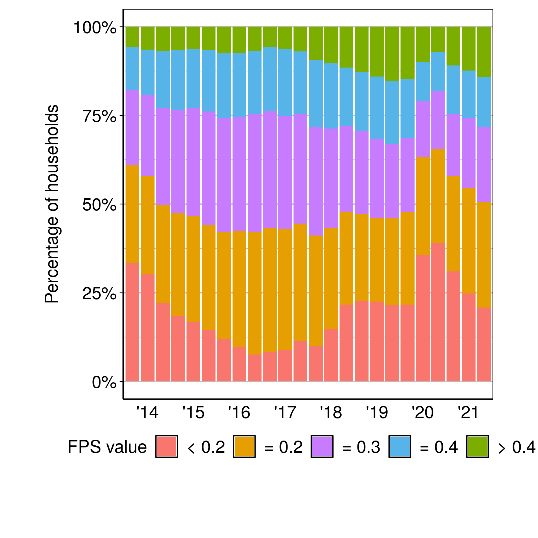
We next examine the cross-sectional variation in household participation. For this, we categorise all households into five groups: those with (1) FPS less than 0.2, (2) equal to 0.2, (3) equal to 0.3, (4) equal to 0.4, and (5) greater than 0.4. Figure 1 shows the fraction of households in each of these FPS categories, in each wave.

Figure 1: Distribution of households by categories of FPS

Figure 1 shows that there was an increase in household financial participation in the early part of this sample, from 2014 up until the end of 2017. (The areas under the sum of FPS categories >= 2 have dropped in this period.) In 2018 and 2019, there was no change in the fraction of households across the defined categories. The changes of 2014-2016 appear to reverse from the second half of 2020 onwards. By 2021, the fraction of households with FPS >= 0.3 is nearly the same as the values seen in 2019.

What was happening at the level of the individual instruments?

In Figure 2, we go below the aggregate FPS into portfolio of individual instruments, including bank accounts, fixed deposits, pensions, post office savings, health insurance, life insurance, mutual funds and listed shares. (We do not include the household holdings of KVP and NSC because these fractions were very small compared to the selected eight instruments in the figure.)

Figure 2: Distribution of households portfolio of individual financial instruments by wave (log scale)

Health insurance had the highest growth (10 percent of households holding to 40 percent of households holding in the sample in a wave). At the same time, life insurance saw a drop (from 60 percent of households holding to 40 percent of households in the sample holding this in a wave). Post office savings saw an increase (from 8.5 percent of household holding to nearly 20 percent of households holding) while pensions saw a decrease (from 25 percent of household holding to around 18 percent). While the numerical values are small, there was strong growth in mutual funds and listed shares.

How different is financial inclusion for rural vs. urban households?

How does the financial participation of urban households compare to rural households? In the following Figure 3, we examine the distribution of rural and urban households in the four FPS categories presented in Figure 1.

Figure 3: Distribution of rural and urban households by categories of FPS

The figures show that the distribution of rural households tend to have lower financial inclusion compared to the urban households. More interesting is the difference in the evolution of financial inclusion between these two groups. Both rural and urban households saw increasing financial participation in 2015 and 2016 compared to 2014. However, financial participation of rural households stalled at the end of 2016, while urban households contend to grow their financial participation. Financial participation for both rural and urban households worsened first in 2018, and then more sharply in 2020, at the time of the pandemic.

We also examine what are the differences in financial instruments holdings behind the variation that we see in the financial participation of rural and urban households. From Figure 4, we can see that rural and urban households are similar in their holding of bank accounts, fixed deposits and post office savings. But they are distinctly different in their holding of EPF, mutual funds and listed shares, where there is a higher fraction of urban households holding these instruments compared to rural households.

Figure 4: Distribution of rural and urban households' portfolio of individual financial instruments

Figure 4 also shows us that the growth in fraction of households holding individual instruments vary between rural and urban households. There was a higher growth in fraction of rural households holding health insurance (from 5 to 40 percent), while for urban households this was lower (from 10 percent to 40 percent). There was a drop in the fraction of rural households holding life insurance compared to no change in the fraction of urban households holding these.

This tells us two pertinent aspects of the growth of financial participation across rural and urban households: first, financial participation by rural households appear more vulnerable to external shocks -- such as demonetisation, the ILFS-NBFC crisis and the pandemic -- than urban households. Second, there is some variation in what types of instruments rural households tend to hold compared with urban households.

In the CPHS sampling strategy, there is a roughly two-times over-weighting of urban locations. The simple summary statistics shown in this article (i.e. unweighted estimates) are problematic; for more precise estimates all summary statistics require appropriate weighting. It is hence particularly useful to see the urban and rural values separately, as has been done here.

Conclusions

It is widely believed that improvements in financial inclusion will translate into reductions of consumption volatility and increased odds of improved lives. Greater research is required on measuring the strength of these relationships. In the standard recipe of phenomenological research, we require measurement of a phenomenon, and then it becomes possible to analyse the causes and consequences.

An important missing link in the field of financial inclusion are tools for measurement. In this article, we have shown a first and simplest measure, an input measure, about use of the formal financial system by households. This measure can be computed at the household level, three times a year, in the CMIE CPHS survey database.

In the summary statistics shown here, there have been only small changes in the overall average FPS over the years under examination. The median value for urban households was 0.3 and the median value for rural households was 0.2. We see a visible decline of the FPS in the lockdowns of 2020, and in the post-pandemic economic recovery, the FPS has come back to near pre-pandemic values. These results suggest numerous questions about causes and consequences, which need to be explored in downstream research.

This ability to observe the FPS at the level of a household enables new kinds of academic research, new kinds of feedback loops for policy makers, and definitions and measurement to help ESG investors overcome principal-agent problems between the investor and the fund, and the fund and the portfolio company.

References:

Andersen, S., Campbell, J. Y., Nielsen, K. M., & Ramadorai, T. (2020). Sources of inaction in household finance: Evidence from the Danish mortgage market, American Economic Review, 110(10), 3184-3230.

Badarinza, C., Campbell, J. Y., & Ramadorai, T. (2016). International comparative household finance, Annual Review of Economics, 8, 111-144.

Banerji, R., Bhattacharjea, S., & Wadhwa, W. (2013). The annual status of education report (ASER), Research in Comparative and International Education, 8(3), 387-396.

Beck, T. (2016). Financial Inclusion–Measuring progress and progress in measuring.

Calvet, L. E., Campbell, J. Y., & Sodini, P. (2007). Down or out: Assessing the welfare costs of household investment mistakes, Journal of Political Economy, 115(5), 707-747.

Campbell, J. Y. (2006). Household finance, The Journal of Finance, 61(4), 1553-1604.

El-Zoghbi, M. (2019). Toward a New Impact Narrative for Financial Inclusion, CGAP, 2019.

Gupta, S., & Sharma, M. (2021). A Demand-Side Approach to Measuring Financial Inclusion: Going Beyond Bank Account Ownership, Dvara Research Working Paper Series No. WP-2021-05.

Monsura, M. P. (2020). The importance of financial literacy: Household's income mobility measurement and decomposition approach., The Journal of Asian Finance, Economics and Business, 7(12), 647-655.

Nguyen, T. T. H. (2021). Measuring financial inclusion: a composite FI index for the developing countries , Journal of Economics and Development, Volume 23, Number 1, pp. 77-99, 2021.

Nilekani N (2019). Report of the High Level Committee on Deepening of Digital Payments, Reserve Bank of India.

Rao, K. S. (2018). Financial inclusion in India: Progress and prospects , The Ideas for India blog, 2018.

RBI (2017). Report of the Household Finance Committee on Indian Household Finance, 24 August 2017.

RBI (2020). National Strategy for Financial Inclusion 2019-2024 .

Sarma, M. (2008). Index of financial inclusion Working paper No. 215, ICRIER, New Delhi.

Sarma, M. (2016), Measuring financial inclusion using multidimensional data, World Economics, 1 Ivory Swuare, Plantation Wharf, London, UK, SW11 3UE, vol. 17(1), pages 15-40, January 2016.

International Finance Corporation (IFC) (2011). Financial inclusion data: assessing the landscape and country-level target approaches. The World Bank, 2011.

United Nations Environment Program Finance Initiative (UN EPFI) (2021). 28 Banks collectively accelerate action on universal financial inclusion and health, 2 December 2021

Geetika Palta, Mithila Sarah and Susan Thomas are researchers at the XKDR Forum. We thank Ajay Shah and three anonymous referees for valuable comments and suggestions.