The Leap Blog

Wednesday, July 13, 2022

Identifying roadblocks in highway contracting: lessons from NHAI litigation

Introduction

Government contracting is an important foundational process which shapes state capacity. Under Indian conditions, there is limited state capacity in government contracting, which leads to a significant rate of contracting failure. One manifestation of contracting failure is litigation. Defects in the contracting process are often associated with litigation. In addition, litigation leads to delays in project completion, and the prospect of litigation deters some private firms from working with government thus hampering competitiveness in government contracting (Mehta and Uday, 2022). The study of litigation is, therefore, a pathway to creating knowledge in the field of government contracting. An example this was Damle et al, 2021.

In the `contract life cycle approach', government contracting is a pipeline that runs through four phases: I - Contract design, II - Contract award, III - Contract management and IV - Contract closure. We must measure the incidence of defects across the four phases, so as to prioritise resourcing, in the field of policy research, and in the activity of government contracting.

In this article, we construct a novel data-set about contract related litigation at the National Highways Authority of India (NHAI), which is the single agency that does the largest number of government contracts. Using this data-set, we measure the share of each of the phases of the procurement life-cycle in litigation. In our knowledge, this constitutes the first empirical evidence about the role of the phases of the government contracting life cycle in inducing litigation.

Methodology

We hand-construct a data-set which draws upon information from three sources.

Delhi High Court case orders: NHAI contracts and concession agreements give the Delhi High Court exclusive jurisdiction over its contractual disputes from anywhere in India. We find 1165 cases in 2007-2020 that emanate from NHAI contracts. For each case, we observe the date of initiation and disposal, and the names of parties involved.
Extracting facts from court documents: We read 635 out of the 1165 (65 percent) court documents. Using these, we extracted the cause of dispute whenever it was available. These were found to be one of the following: Interim relief, Appointment of arbitrator, Challenging arbitration award, Seeking extension of time, Seeking award enforcement, Restraining NHAI, Reimbursement of costs/Compensation, Challenging claims demanded.
The NHAI Draft Red Herring Prospectus (DRHP): While filing for the NHAI Infrastructure Investment Trust listing with SEBI, MoRTH was mandated to disclose all large-value disputes involving the NHAI (that are in arbitration), along with a list of all outstanding claims. This had 40 disputes listed, with information about the dates of initiation, cause of disputes, the model of contracting used for the project under dispute, and the names of parties involved. As a self-disclosed data source, this served as a tool to validate observations from the Delhi High Court case orders data.

We find that NHAI accounts for almost 40% of the cases that the Union Government is party to (1165 out of the Union Government's 2912). We also find that cases involving the NHAI have grown at a rate of 17.15% on average during this period. NHAI is the petitioner for about 45% of the cases, while the corresponding figure for other government agencies is about 30%.

NHAI is such a large scale litigant, that reducing the litigation intensity at NHAI would make a different to the working of the judiciary. This work is thus relevant not just for the field of government contracting, but also for the field of the judiciary.

We develop a two-step process for classifying NHAI contract related litigation orders into the four phases of the government contracting life cycle. In the first step, we categorise cases based on causes of dispute as follows:

Related to arbitration proceedings: One set of cases pertain to petitions that (1) seek interim relief from the court under Section 9 of the Arbitration and Conciliation Act 1996, (2) seek the court's intervention in selection of the arbitrator (on account of delays or disagreement in appointment), and (3) appeal awards announced by the arbitral tribunal, which accounted for a significant fraction of the arbitration related matters.
Payments related: This could be about payments, revision of payment terms, price estimation due to changes in scope/ additional components midway into the construction phase or changes in law or policy leading to adverse conditions of work for the private party. Changes in terms of the contract result in parties disagreeing over revised cost estimates or the method of calculating these revisions. In several cases, the delays were related to reimbursements to the private party on account of delays in land acquisition, or operationalising toll plazas. In some cases, the private firm sought restraining orders from the court against the NHAI invoking bank guarantees when there was a delay in the firm achieving financial closure.
Related to wrongful termination/debarment of contractors: Concession agreements embed the terms of contract termination. Prior to the 2020 amendment in the model concession agreement (which allowed a mutual exit clause), the contract perceived termination as default by either side, with the opposite party having a right to compensation and damages. In the process, NHAI often debarred/black-listed contractors from bidding for tenders, a decision that contractors appeal in court.
Reason unclear: For 253 cases, we were unable to classify the cause of dispute since the order was unclear for interpretation. This may reflect blemishes in the Delhi High Court website. We are conservative and classify a case under `Reason unclear' when we are not confident about placing it into the other three categories.

We go on to classify cases into the four phases of the life-cycle of a contract. This mapping is sensitive to the domain; our classification processes are specific to government contracting in highways and infrastructure.

In all the cases that we studied, there was none in the first phase (the "Contract design" phase).

Litigation associated with defects in the pre-award phase involves disputes on the tendering/awarding processes. For example, this includes disputes regarding unfairly awarded tenders, wrongly classifying bids as non-responsive and irregular financial bid-opening processes, all of which are placed within the pre-award phase.

Reading the orders shows that arbitration-related and payments-related causes of disputes take place once the contract has been awarded. This is also true for some of the cases that are classified as wrongful debarment/termination which arises because of the non-performance of contractual obligations. Since these disputes arise after the contract is awarded, we classify these cases in the post-award phase. Some of the orders contain details about the type of contract between the parties. For example, SPVs are often formed for the construction of a highway, and are named '... Tollway Pvt. Ltd.' which indicates a legal entity that was formed for the purposes of executing a contract or an award. This can be identified from the names of the parties, even if the specific causes of dispute might be unclear in some cases. We use this information in classifying cases under the post-award category.

Traditionally, cases pertaining to payment delays are categorised within the post-completion phase. But in the case of NHAI contracts, payment schedules vary across the commonly used models of Hybrid Annuity (HAM), BOT-Annuity models and EPC. Payments are made to the concessionaire either at the start of construction, or at regular frequencies such as semi-annually, with payments usually linked to the achievement of project milestones. We place such cases in the post-award phase rather than in the post-completion phase. Similarly, case orders that seek to resolve arbitration-proceedings related disputes are also categorised as post-award since these disputes arise from a contractual relationship between two parties to approach alternate dispute resolution mechanisms, which can only exist in the event of a contract being awarded.

Findings

Table 1: Number of cases by drivers of litigation

Cause of dispute	NHAI as petitioner	Firm as petitioner	Total
Arbitration proceedings related	123	137	260
Payments related	15	75	90
Wrongful termination/ debarment	1	31	32
Total	139	243	382

In Table 1, we summarise the number of cases falling under Categories 1-3 listed above. We further break up the cases under each category as the number of cases where NHAI was the petitioner and where the private firm was the petitioner. A large volume of cases are a) arbitration-proceedings related, and 2) payments-related (delayed payments). We see that arbitration related matters are nearly 70 percent of the sample of case orders. In this category, both the NHAI and the firm are almost equally likely to petition an arbitration matter. In the other two categories, NHAI is more likely to be litigated against.

The analysis based on case classification into phases of the contract life-cycle is presented in Table 2. This shows the number of disputes which we classify as falling within the pre-award, post-award, and post-completion phase. In this table, we present both the actual number of cases identified in a given phase, as well as the share of the cases as a fraction of the total.

Table 2: Share of disputes by the phase of the contract life-cycle

Phase of the contract life-cycle	Share (% of Total)	Number of cases
Pre-award	1.75	11
Post-award	66.14	420
Post-completion	0.15	1
Unclear/No data recorded	31.95	203
Total	100.00	635

Table 2 shows that over 65% of the cases are concentrated in the post-award or the contract management phase.

Discussion

In this article, we have analysed one important government contracting organisation, and attributed its litigation into the four phases of the contract life cycle. The results diverge from the commonly held view that the problems in public procurement arise because of problems with Phase 2 or L1 tendering. This analysis suggests that the hot spot in litigation is Phase 3 or the Contract management phase. This suggests that policy researchers and policy practitioners should allocate greater resources on strengthening this phase.

Another finding is that there is a large volume of arbitration-proceedings related disputes, which indicates the limitations of alternate dispute resolution (ADR) mechanisms. Strengthening ADR mechanisms in India would result in less litigation.

Recent reforms of the government contracting process have initiated movement on this front. The General Instructions on Procurement and Project Management (2021) built provisions to address concerns around arbitration and dispute resolution. It acknowledges that the majority of the cases appealed by government agencies end up being awarded in favour of the opposite party. In this context, the General Instructions emphasize the need for the government to actively take steps to minimise litigation. Further, it inserts Rule 227A in the General Financial Rules (GFRs) 2017 for Arbitration Awards, which mandates that the concerned ministry pay 75% of the amount of the arbitral award against the bank guarantee, even if it contests the award in a court of law. This is a step in the right direction as it takes away the incentive for either party to benefit from prolonging a dispute or appealing to a higher authority to delay payment of claims awarded by the arbitral tribunal.

References:

Damle D., Gulati K., Sharma A., and Zaveri-Shah, B. Litigation in public contracts: some estimates from court data., The LEAP Blog, May 2021.

Mehta C., and Uday D., How competitive is bidding in infrastructure public procurement? A study of road and water projects in five Indian states, The LEAP Blog, March 2022.

Charmi Mehta is a researcher at XKDR-Chennai Mathematical Institute and Susan Thomas is professor at the Jindal School of Business and a researcher at XKDR Forum. The authors thank Shailesh Pathak and Bhargavi Zaveri-Shah for their inputs in shaping the study, and Yajat Bansal and Diya Mal for their research assistance in this study.

Sunday, July 03, 2022

Measuring financial inclusion: how much do households participate in the formal financial system?

by Geetika Palta, Mithila A. Sarah and Susan Thomas.

Measuring the impact of financial inclusion

Households use financial instruments and financial markets to achieve their lifetime objectives. These include being able to smooth consumption over time, being able to withstand shocks, and pursue entrepreneurial opportunities to gain income mobility. Financial inclusion refers to such access to finance for a larger subset of the population (e.g. Rao, 2018). Financial policy makers have pursued financial inclusion for many decades. In recent years, the rise of ESG investors has bolstered private sector interest in financial inclusion.

For policy makers, for financial firms, and for ESG investors, there is thus an interest in the measurement of financial inclusion (Sarma M., 2016; UNEP FI, 2021). The field of measurement of financial inclusion is under-developed. While there is high interest in building such measures (RBI, 2020; El-Zoghbi, 2019), there are debates about methods and no single measure has been widely accepted (Nguyen, 2021).

Financial inclusion should improve the life of the household through smoothing consumption, withstanding shocks to income and helping the household achieve income mobility to a higher sustained level of consumption. For example, learnings from a financial literacy program in the Philippines show how Filipino households obtained income mobility (Monsura, 2020). These households learned how to take advantage of the economic opportunities through savings, investment, insurance, and entrepreneurship. Access to formal financial services and the ability to use them enables the households build wealth and generally live a financially secure life.

An inputs-outputs-outcomes framework

The inputs-outputs-outcomes framework is valuable in many aspects of policy thinking. As an example, in a domain like education, the input is school buildings, the output is children spending hours in school, and the outcome is the change in their knowledge (Banerji et al., 2013).

This approach is valuable in the field of financial inclusion also. The input is household participation in formal finance (such as account opening or purchasing health insurance); the output is the intensity of transactions (how frequently the account is used or whether the insurance premium is paid on a regular basis) and the outcome is the impact on economic well-being.

This perspective upon financial inclusion guides measurement methods for financial inclusion. Measurement of financial inclusion needs to measure inputs (presence of various financial products and services in the household portfolio), outputs (the use of financial products in achieving household objectives) and outcomes (stability of consumption and income mobility).

Done right, such measures can facilitate a deeper understanding of the impact of financial inclusion on the economic well-being of a household. These measures can help identify gaps in financial inclusion, both in terms of missing products in the household financial portfolios, as well as excluded household groups. For ESG investors, these measures can play a role in their principal-agent problems with portfolio companies.

In this article, we propose and implement a simple financial inclusion input measure, which is the household participation in the formal financial sector, calculated using the sample of households in the CMIE CPHS data. With this, we show some important facts about financial inclusion inputs in India.

Difficulties of conventional measures

In the early stages of measuring financial inclusion, crude proxies were used for measurement at the level of the economy, such as M2 (cash, demand and time deposits) as a percentage of GDP. Later, more systematic data collection about household holdings of financial assets began (Beck, 2016). Most of these measures were typically country-level aggregates organised around financial service provider (FSP) or one class of financial product (RBI, 2017). While aggregates at the country level are useful, they can mix up usage by some households and absence by others. What would be most useful is to construct financial inclusion measures at the level of a household, pulling together a full picture of the financial activities of the household (Campbell, 2006).

More often than not, there has been a bank-orientation in these measures with focus on number of bank accounts, bank branches, number of ATMs and amount of bank deposits. But there is much more to financial inclusion than banking. Gupta and Sharma (2021) point out that measuring ownership of bank accounts alone tends to overestimate and present an incomplete picture of financial inclusion as it neglects access to and use of the full range of financial products. Over time, the focus of financial inclusion has shifted towards a larger set of financial assets and usage of digital payment systems (RBI, 2020).

The construction of financial inclusion measures at the level of a household pre-require a capture of such information from households themselves. There are a few rare instances where countries have administrative data from which asset portfolio by households can be constructed (Calvet et al., 2007; Andersen et al., 2020). Most countries do not have such data on household portfolio of financial instruments (Badarinza et al., 2016; IFC, 2011). Over the last decade or so, household surveys have emerged that record household portfolio of financial instruments. Most of these have been one time surveys or surveys done at low frequencies. For example, in India, the NSSO AIDIS captures household level participation in financial systems once in 10 years.

Constructing a household `Financial Participation Score' (FPS) using CPHS

An important household survey that is conducted thrice a year over a sample of 170,000 households is the Consumer Pyramids Household Survey (CPHS), by the Centre for Monitoring Indian Economy. Given India's high economic growth rate and the rapid pace of change in the last few decades in finance, this survey makes possible new insights into financial inclusion of Indian households in a timely and geographically dis-aggregated manner.

The CPHS has member-wise characteristics and household characteristics such as income and expenditure of households, what assets they own and whether they have borrowings. Household data on financial assets owned comes from the ''People of India database'' and the ``Household Aspirational India database'' in CPHS. In the former, households are asked questions on ownership (Yes/No) of four different financial instruments, while the latter measures outstanding investment (Yes/No) in six financial instruments. We use the following variables to measure the financial participation of a household:

Household ownership of at least one bank account (Bank), at least one health insurance (HI), at least one life insurance (LI), at least one employee provident fund account (EPF).
This captures four components of financial inclusion.
Outstanding investment at a household level in fixed deposit (FD), Kisan Vikas Patra (KVP), National Savings Certificate (NSC), Post Office Savings account (POS), Mutual Funds (MF) and Listed Shares (LS).
This captures six components of financial inclusion.

Put together, there is data about 10 financial instruments -- all zero/one values -- that households hold at a point in time. We define a Financial Participation Score as sum of the values divided by 10. This gives the household an FPS that runs from 0 to 1. For example, an FPS value of 0.3 indicates that the household owns three of the ten financial instruments.

The CPHS data on household holding of the 10 financial instruments is captured three times a year in three ``waves'' where each wave is completed over four months and surveys about 170,000 households. In each year, Wave 1 consists of January, February, March, April 2021; Wave 2 has May, June, July, August and Wave 3 has September, October, November and December. Households are generally measured in a consistent month slot within each wave thus generating a regular cadence in the time-series for each household.

All the 10 instruments used in this calculation involve households carrying consumption from the present into the future. In this article, we do not include debt-related variables in calculating financial participation, even though borrowing is one form of finance used by many households. For one, debt is multi-dimensional. It can be from different sources (formal vs. informal), have different maturities, be driven by different purposes. While all debt involves carrying consumption from the future to the present, the impact of debt on the future well-being of the household can vary. Some debt is for short-term consumption smoothing, possibly at the cost of lower consumption in the future. Other types of debt may lead to higher income in the future if they are used to build enterprise. Given this multi-faceted nature of household debt, it's inclusion is left for downstream research.

We construct an unbalanced panel data-set of household FPS at the wave level, for 2014-2021, with three waves per year. The number of households observed varies from 76,386 (during the lock-down in 2020) to 1,49,160 (2018). The CPHS is a stratified random sample. However, for the purpose of this first exploration of basic facts, we have reported unweighted summary statistics.

Some basic facts about the FPS

The household FPS is calculated for each wave. The annual FPS of a household is calculated as the maximum value of FPS observed for the household across all the waves for which it was observed. The summary statistics of annual household FPS values are presented in Table 1 for each year of the panel data-set.

Table 1: Summary statistics of household FPS, from 2014 to 2021

	2014	2015	2016	2017	2018	2019	2020	2021
Min	0.0	0.0	0.0	0.0	0.0	0.0	0.0	0.0
25th	0.1	0.2	0.2	0.2	0.2	0.2	0.2	0.1
50th	0.2	0.3	0.3	0.3	0.3	0.3	0.3	0.2
75th	0.3	0.3	0.4	0.3	0.4	0.4	0.4	0.3
Max	0.9	0.9	1.0	1.0	1.0	1.0	1.0	0.9

For most of the years, 50 percent of the households hold 3 or fewer instruments. This holds steady for the 6 year period, for most part. There continue to be households with FPS of 0. This implies that there continue to be households that do not even have bank accounts in this sample.

There have been minor shifts in financial participation of the households in this period. The COVID-19 pandemic lock down of April to June 2020 appears to have an adverse impact. By 2021, the median household has dropped from holding 3 instruments to 2. This is a consistent drop -- the 25th percentile household have dropped from 2 to 1 instrument, and the 75th percentile household has gone down from 4 to 3.

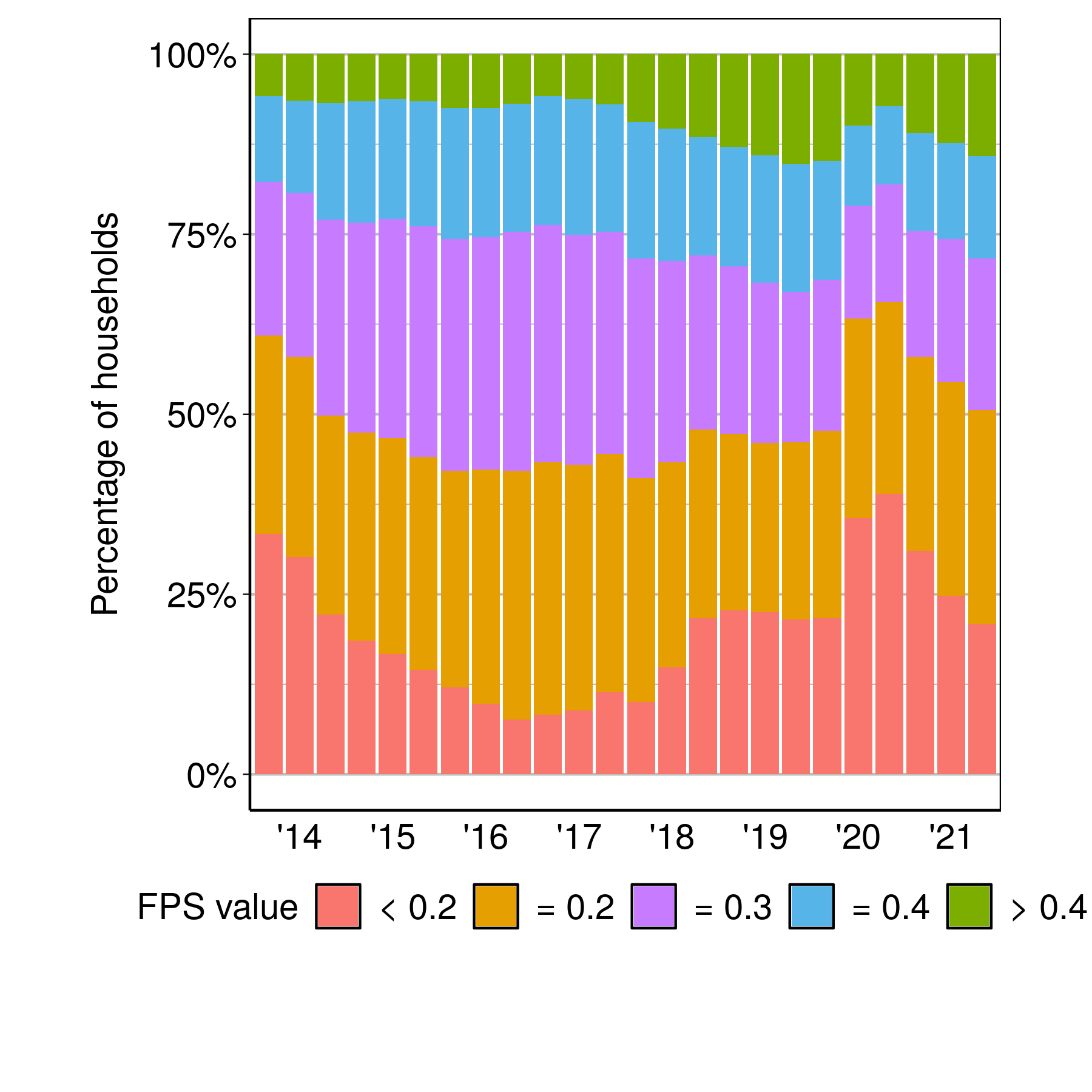
We next examine the cross-sectional variation in household participation. For this, we categorise all households into five groups: those with (1) FPS less than 0.2, (2) equal to 0.2, (3) equal to 0.3, (4) equal to 0.4, and (5) greater than 0.4. Figure 1 shows the fraction of households in each of these FPS categories, in each wave.

Figure 1: Distribution of households by categories of FPS

Figure 1 shows that there was an increase in household financial participation in the early part of this sample, from 2014 up until the end of 2017. (The areas under the sum of FPS categories >= 2 have dropped in this period.) In 2018 and 2019, there was no change in the fraction of households across the defined categories. The changes of 2014-2016 appear to reverse from the second half of 2020 onwards. By 2021, the fraction of households with FPS >= 0.3 is nearly the same as the values seen in 2019.

What was happening at the level of the individual instruments?

In Figure 2, we go below the aggregate FPS into portfolio of individual instruments, including bank accounts, fixed deposits, pensions, post office savings, health insurance, life insurance, mutual funds and listed shares. (We do not include the household holdings of KVP and NSC because these fractions were very small compared to the selected eight instruments in the figure.)

Figure 2: Distribution of households portfolio of individual financial instruments by wave (log scale)

Health insurance had the highest growth (10 percent of households holding to 40 percent of households holding in the sample in a wave). At the same time, life insurance saw a drop (from 60 percent of households holding to 40 percent of households in the sample holding this in a wave). Post office savings saw an increase (from 8.5 percent of household holding to nearly 20 percent of households holding) while pensions saw a decrease (from 25 percent of household holding to around 18 percent). While the numerical values are small, there was strong growth in mutual funds and listed shares.

How different is financial inclusion for rural vs. urban households?

How does the financial participation of urban households compare to rural households? In the following Figure 3, we examine the distribution of rural and urban households in the four FPS categories presented in Figure 1.

Figure 3: Distribution of rural and urban households by categories of FPS

The figures show that the distribution of rural households tend to have lower financial inclusion compared to the urban households. More interesting is the difference in the evolution of financial inclusion between these two groups. Both rural and urban households saw increasing financial participation in 2015 and 2016 compared to 2014. However, financial participation of rural households stalled at the end of 2016, while urban households contend to grow their financial participation. Financial participation for both rural and urban households worsened first in 2018, and then more sharply in 2020, at the time of the pandemic.

We also examine what are the differences in financial instruments holdings behind the variation that we see in the financial participation of rural and urban households. From Figure 4, we can see that rural and urban households are similar in their holding of bank accounts, fixed deposits and post office savings. But they are distinctly different in their holding of EPF, mutual funds and listed shares, where there is a higher fraction of urban households holding these instruments compared to rural households.

Figure 4: Distribution of rural and urban households' portfolio of individual financial instruments

Figure 4 also shows us that the growth in fraction of households holding individual instruments vary between rural and urban households. There was a higher growth in fraction of rural households holding health insurance (from 5 to 40 percent), while for urban households this was lower (from 10 percent to 40 percent). There was a drop in the fraction of rural households holding life insurance compared to no change in the fraction of urban households holding these.

This tells us two pertinent aspects of the growth of financial participation across rural and urban households: first, financial participation by rural households appear more vulnerable to external shocks -- such as demonetisation, the ILFS-NBFC crisis and the pandemic -- than urban households. Second, there is some variation in what types of instruments rural households tend to hold compared with urban households.

In the CPHS sampling strategy, there is a roughly two-times over-weighting of urban locations. The simple summary statistics shown in this article (i.e. unweighted estimates) are problematic; for more precise estimates all summary statistics require appropriate weighting. It is hence particularly useful to see the urban and rural values separately, as has been done here.

Conclusions

It is widely believed that improvements in financial inclusion will translate into reductions of consumption volatility and increased odds of improved lives. Greater research is required on measuring the strength of these relationships. In the standard recipe of phenomenological research, we require measurement of a phenomenon, and then it becomes possible to analyse the causes and consequences.

An important missing link in the field of financial inclusion are tools for measurement. In this article, we have shown a first and simplest measure, an input measure, about use of the formal financial system by households. This measure can be computed at the household level, three times a year, in the CMIE CPHS survey database.

In the summary statistics shown here, there have been only small changes in the overall average FPS over the years under examination. The median value for urban households was 0.3 and the median value for rural households was 0.2. We see a visible decline of the FPS in the lockdowns of 2020, and in the post-pandemic economic recovery, the FPS has come back to near pre-pandemic values. These results suggest numerous questions about causes and consequences, which need to be explored in downstream research.

This ability to observe the FPS at the level of a household enables new kinds of academic research, new kinds of feedback loops for policy makers, and definitions and measurement to help ESG investors overcome principal-agent problems between the investor and the fund, and the fund and the portfolio company.

References:

Andersen, S., Campbell, J. Y., Nielsen, K. M., & Ramadorai, T. (2020). Sources of inaction in household finance: Evidence from the Danish mortgage market, American Economic Review, 110(10), 3184-3230.

Badarinza, C., Campbell, J. Y., & Ramadorai, T. (2016). International comparative household finance, Annual Review of Economics, 8, 111-144.

Banerji, R., Bhattacharjea, S., & Wadhwa, W. (2013). The annual status of education report (ASER), Research in Comparative and International Education, 8(3), 387-396.

Beck, T. (2016). Financial Inclusion–Measuring progress and progress in measuring.

Calvet, L. E., Campbell, J. Y., & Sodini, P. (2007). Down or out: Assessing the welfare costs of household investment mistakes, Journal of Political Economy, 115(5), 707-747.

Campbell, J. Y. (2006). Household finance, The Journal of Finance, 61(4), 1553-1604.

El-Zoghbi, M. (2019). Toward a New Impact Narrative for Financial Inclusion, CGAP, 2019.

Gupta, S., & Sharma, M. (2021). A Demand-Side Approach to Measuring Financial Inclusion: Going Beyond Bank Account Ownership, Dvara Research Working Paper Series No. WP-2021-05.

Monsura, M. P. (2020). The importance of financial literacy: Household's income mobility measurement and decomposition approach., The Journal of Asian Finance, Economics and Business, 7(12), 647-655.

Nguyen, T. T. H. (2021). Measuring financial inclusion: a composite FI index for the developing countries , Journal of Economics and Development, Volume 23, Number 1, pp. 77-99, 2021.

Nilekani N (2019). Report of the High Level Committee on Deepening of Digital Payments, Reserve Bank of India.

Rao, K. S. (2018). Financial inclusion in India: Progress and prospects , The Ideas for India blog, 2018.

RBI (2017). Report of the Household Finance Committee on Indian Household Finance, 24 August 2017.

RBI (2020). National Strategy for Financial Inclusion 2019-2024 .

Sarma, M. (2008). Index of financial inclusion Working paper No. 215, ICRIER, New Delhi.

Sarma, M. (2016), Measuring financial inclusion using multidimensional data, World Economics, 1 Ivory Swuare, Plantation Wharf, London, UK, SW11 3UE, vol. 17(1), pages 15-40, January 2016.

International Finance Corporation (IFC) (2011). Financial inclusion data: assessing the landscape and country-level target approaches. The World Bank, 2011.

United Nations Environment Program Finance Initiative (UN EPFI) (2021). 28 Banks collectively accelerate action on universal financial inclusion and health, 2 December 2021

Geetika Palta, Mithila Sarah and Susan Thomas are researchers at the XKDR Forum. We thank Ajay Shah and three anonymous referees for valuable comments and suggestions.

Wednesday, June 15, 2022

Reconsidering SEBI disgorgement

by Renuka Sane and S. Vivek.

SEBI disgorgement is a regulatory remedy to recover wrongful gains from entities that have violated securities laws. It is justified based on the equitable principle that no one should benefit from their own wrong. This seems like a non-controversial, even obvious, ground for regulatory action that has 'compelling intuitive appeal'. However, there are basic conceptual issues that are not clearly settled, not just India but in other jurisdictions as well. For example, the U.S. Supreme Court has considered three cases on disgorgement over the last few years - in one case, it held that disgorgement was beyond the powers of the Federal Trade Commission, overruling decades worth of practice, and in another, upheld Securities and Exchange Commission's power to seek disgorgement but with important conceptual restrictions.

These are trends that the Securities and Exchanges Board in India (SEBI) should be watching carefully. Lack of conceptual clarity about the remedy can put years of regulatory action at risk, if the basis of the remedy is questioned in a case before superior Courts. Further, a study of how SEBI orders are interpreting disgorgement powers and if they are consistent with the conceptual justifications is critical. SEBI disgorgement does not have any statutory limit - the order can direct recovery of all the wrongful gain, whatever they may be. This exercise of of vast discretion by SEBI Whole-Time Members (who are executive members of the regulator and typically do not have substantial judicial training), without transparent statutory or conceptual guidance, raises regulatory governance concerns.

In a new working paper, Reconsidering SEBI disgorgement, we study disgorgement from three perspectives:

The theory of disgorgement: Disgorgement is a distinct remedy that must be distinguished from other remedies such as compensation, restitution, and penalties. Disgorgement is different from compensation because compensation is focussed on the loss suffered by claimants whereas disgorgement is focussed on the gains made by the wrongdoer. While disgorgement and restitution are both gain-based remedies, there is a subtle yet important difference. Restitution is focused on reversing a wrongful gain of the defendant based, for example, on a wrong or incorrect transfer from the plaintiff. Here, the (wrongful) gain made by the defendant is equal to the loss suffered by the plaintiff - the property in question (money, for example), is returned to status quo. Disgorgement, on the other hand, strips the defendant of its gains, even if such gains are not made from the plaintiff, and even if the plaintiff does not suffer any loss. Accordingly, the loss suffered by the plaintiff need not correlate to the defendant's gain that is clawed back through disgorgement. The objective for disgorgement is to have a deterrence effect, and not to merely reverse an illegal transfer. Penalties are also generally imposed for the purpose of deterrence, among others. However, while disgorgement amounts must be equal to the gains made by the wrongdoer, penalties can be imposed merely on the basis of the violation and need not correlate exactly to the gains, if any, made by the wrongdoer.

The evolution of disgorgement at SEBI: SEBI had even in the early years tried exercising powers to claw back illegal gains (disgorgement), or compensate victims in insider trading cases, with mixed success at appellate fora. Subsequently, parliamentary and expert committees over the years have recommended providing SEBI with clear powers to trace the illegal gains made by wrongdoers and return such gains to their victims. Before such powers could be formalised through statute, disgorgement was used by SEBI Whole-Time Members (WTMs) as a quasi-judicial innovation in their orders,and received approval from the Securities Appellate Tribunal. Since, at that time, SEBI WTMs did not have the power to impose monetary penalties, SEBI disgorgement was justified as a 'remedial' power which only returns the wrongdoer to status quo, and hence can be distinguished from a punishment. Further, as there was no express statutory provision at the time for SEBI disgorgement, it was traced back to 'equitable' powers of SEBI WTMs.

In 2014, the Securities and Exchange Board of India Act, 1992 (SEBI Act), was amended to clarify that SEBI disgorgement was part of SEBI's remedial powers. The amendment also stated that the amounts so clawed back are not to be deposited with the Consolidated Fund of India as in the case of penalties; instead, they are retained by SEBI's Investor Protection and Education Fund, to be used in terms of SEBI's own regulations. Interestingly, despite tracing its origins to Parliamentary and expert committees which discussed disgorgement powers in the context of using the proceeds to compensate victims, the amendment did not require SEBI to even attempt to distribute the amounts to victims. Since then, SEBI's power to direct disgorgement without clear statutory limits has been entrenched. Gradually, SEBI also received judicial recognition for its power to impose interest on the disgorgement amount. These rates are calculated from the date of the violation, sometimes going back 10 years or more (as opposed interest on penalties which is typically calculated from the date of non-payment after the SEBI order). Further, the initiation of proceedings for disgorgement or penalties, remains with SEBI and it is unclear how it is exercised.

These vast powers are conferred on the regulator on the basis that SEBI disgorgement is only 'remedial' and is returning the wrongdoer to status quo. The use of the term 'disgorgement' while at the same time emphasising the return to status quo creates some confusion between the related albeit distinct remedies of disgorgement and restitution. In this context, we study whether in practice what kind of remedy SEBI disgorgement actually is, regardless of its nomenclature. Further, as a legal matter, returning the wrongdoer status quo is critical as a point of distinction from SEBI penalties; if the wrongdoer is left worse-off, it could be argued that SEBI disgorgement is a penalty by another name.
The practice of disgorgement at SEBI : If SEBI's case for disgorgement is based on clawing back illegal gains and returning the wrong-doer to status-quo, do they actually do so? We use all the SEBI disgorgement orders between January 1, 2018, and July 15, 2021, and find that in 9% of the cases there is no finding that the noticee has made a benefit or avoided a loss, and yet noticees have been ordered to disgorge. In none of the cases is there a finding that the direction brings the noticee back to status-quo and does not leave them worse off - a critical element in the justification for SEBI disgorgement and its characterization as a remedial power. Further, it is interesting that SEBI disgorgement is usually used for insider trading, and fraudulent trading offences, for which the SEBI Act allows penalties to be issued up to three times the profits made. Why is disgorgement, and not penalties, being used in these cases?

Our results suggest that lawmakers and the SEBI Board must review how SEBI disgorgement is conceptualised and what goals it serves. It should scrutinise how disgorgement orders are being issued under the existing framework so that they are consistent with the justifications for remedial measures (such as, allowing deductions for legitimate expenses and a transparent and careful system to determine causation of the gains from the wrong). A holistic look at remedies available for securities law violations is required so that they serve all the goals required for stakeholders - deterrence, compensation, and restitution.

S. Vivek is a researcher with the Regulatory Governance Project at the National Law School of India University, Bengaluru. Renuka Sane is a researcher at NIPFP. Author names are in alphabetical order.

Friday, June 10, 2022

Threats to legal certainty in government contracting by electricity distribution companies

by Akshay Jaitly and Ajay Shah.

A battle in Andhra Pradesh, 2018-2022

In September 2018, electricity distribution companies in Andhra Pradesh (Discoms) filed a petition before the Andhra Pradesh Electricity Regulatory Commission (APERC) to reduce the feed-in tariff for wind power projects (that had been determined under Section 62 of the Electricity Act, where the regulator sets the price). Another petition was filed requesting APERC to revise the tariff payable by Discoms under solar power PPAs (this time discovered under Section 63 of the Electricity Act, where there is a competitive bidding process). The argument made by Discoms was that the tariff discovered in other states pursuant to competitive bidding was lower than the tariffs statutorily determined in Andhra Pradesh. There are also newspaper reports about the state load dispatch centre (SLDC) curtailing output by renewables generators, ostensibly in the interests of grid safety.

These attempts at reneging on contracts, by the state, go against basic notions of sanctity of contracting and legal certainty. When X contracts with Y, both are bound by and obliged to fulfil the terms of the contract, regardless of future fluctuations of prices and technology. The Indian Contract Act, 1872, and a line of case law under it, gives no space for either X or Y, as private persons, to renege on a contract because better prices had come about somewhere else in the economy.

It is also settled law that when the state enters into a contract, it does so in a commercial capacity and not as the sovereign. If the Indian state purports to renege on contracts in this fashion, it deepens the problems of the state as an untrusted counterparty, and fewer private persons will be willing to do business with the state in the future. This would harm the prices at which the state is able to enter into contracts.

As an example, consider a Jan 2022 story by Kailash Babar in the Economic Times, about NHAI terminating a contract with IL&FS which had been established in 2013. NHAI did not just walk away: it paid IL&FS Rs.891 crore for the privilege of terminating the contract. Concessions typically have a formula for termination compensation in three scenarios – authority default, no fault and concessionaire default. These are expressed as percentages of debt due plus some equity return and some other terms.

Attempts at reneging on PPAs elsewhere in India

This experience from Andhra Pradesh is actually not unique. Discoms and regulators in Karnataka, Uttar Pradesh, Jharkhand and Tamil Nadu have subsequently attempted unilateral termination or renegotiation of renewable energy tariffs under validly executed PPAs.

Punjab took this one step further in November last year, by introducing and unanimously passing legislation to get out of its PPA obligations. A few months ago, we wrote about the Punjab Renewable Energy Security, Reform, Termination and Re-Determination of Power Tariff Bill passed in the Punjab Legislative Assembly. This law seeks to renege on PPAs that the Punjab state Discom had voluntarily entered into, on the basis that these created too heavy a financial burden on the state. This attempt by the state, to have immunity from contract performance, is under legal challenge.

A seminal skirmish took place a while ago, in Gujarat in 2013, where the Appellate Tribunal for Electricity had held with reference to the actions of a Discom in Gujarat, that a PPA could only be reopened for "giving thrust to renewable energy projects and not for curtailing the incentives". In other words, PPAs could not be reopened to reduce tariffs. In this case, Gujarat Urja Vikas Nigam Ltd (GUVNL) had filed a petition before the Gujarat Electricity Regulatory Commission (GERC) in 2013, asking for a revision in solar tariffs determined by the commission in its 2010 order on the grounds of reduced customs and excise duties, which would justify a downward revision of the tariffs. The GERC dismissed GUVNL’s petition and its decision was upheld by the Appellate Tribunal for Electricity (APTEL) on appeal. APTEL held that since GUVNL had not established that there is a legal right available to it to seek a redetermination of the tariff by reopening the PPA, the GERC would not be expected to revisit the generic tariff ‘to dis-incentivise the project developers and consequently discourage future investment in the sector’.

How the Andhra Pradesh story played out

Despite this, solar and wind power developers challenged this in the High Court of Andhra Pradesh. A single judge bench of the High Court dismissed the Discoms' petitions in September 2019, with a direction to APERC to decide the issues raised by the developers.

But the High Court directed the Discoms to pay an interim tariff (lower than the tariffs under the PPAs) until APERC adjudicated the matter. The legal foundations through which the court chose to go against contract law are not clear. This created tremendous commercial difficulties in the industry. In some instances, there are reports that even this lower interim tariff was not being paid by the Discoms, causing further distress to power generators.

The typical renewables project is a tight arrangement of capital and PPA, with little room for contracting wobbles. Once the predictability of cash flows was disrupted, some of the generating assets were classified as 'non-performing'. The generators tried to go to court to force lenders to not do so.

This problem then showed up at a Division Bench at the Andhra Pradesh High Court. The case played out over three years. The Division Bench held that:

The tariff under concluded PPAs cannot be re-negotiated;
Financial difficulty of Discoms is not a ground to permit non-performance of the PPAs or to reduce the tariff set out under the PPAs;
A tariff determined through competitive bidding process under Section 63 of the Electricity Act cannot be re-determined; and
Since renewable energy plants operate on a ‘must-run basis’, any arbitrary curtailment of power by the state load despatch centre without notice and not based on grid security or safety reasons is illegal.

This was a salutory reaffirmation of the foundations of commercial law: Contracts must be honoured, statutory processes cannot be unilaterally set aside, power validly contracted under a PPA can only be curtailed for technical reasons. At the same time, in a well functioning market economy, these events from 2018 to 2022 -- and the associated commercial consequences for private persons -- should have never taken place. Every investor looks at this fracas and chooses a somewhat higher risk premium for doing business in India.

Implications for the Indian legal system

It is important to analyse what shapes these attempts at state immunity from contract law. In what ways can laws be amended, or principles be evolved, so that such attempts are eliminated or at least minimised?

Perhaps the Andhra Pradesh Discoms will appeal to the Supreme Court of India in this matter; perhaps the challenge to the Punjab PPA law will find its way to the Supreme Court. It is then interesting to envision: What is the Supreme Court order that can usefully underline the foundations of the extant contract law, and thus reduce the incentives to embark on such manoeuvres?

While a Supreme Court order in this regard might act as a deterrent in the future, the problem lies in the culture of government institutions, who are conditioned to exhaust all available means of reducing costs, irrespective of the merits of their position and the chances of success, out of fear of vigilance authorities. A solution would be for the government to develop guidelines and instructions setting out the bases on which appeals should be pursued or not.

In developing such guidelines, some of the questions for the state to consider would be as follows: Suppose the probability of success of such attempts at renegotiating are 0. Is it still efficient for a state government to initiate it? As Karan Gulati and Shubho Roy emphasise in a forthcoming paper, could it be that the time value of money that is used in Indian court orders make it efficient for the state government to embark on litigation that it has no possibility of winning? We need to also analyse the Indian justice system from this point of view, and identify the reforms through which the incentive of a state government is reshaped.

Implications for electricity policy

As we have argued before, the Indian electricity sector has suffered from difficulties for a long time, but the recent years represent an escalation of stress to a different level. This comes from the combination of low price renewables, volatility in fuel costs, the impact of ESG investors abroad upon electricity purchase by large Indian firms, and the accelerating exit of commercial and industrial buyers from discoms.

It is sometimes comforting to think that discoms in India have always had problems. But the problems seen today are worse. Faced with extreme stress, there is an appetite for extreme measures. When the policy process is weak, there is a greater likelihood of poorly designed policy measures being adopted, such as attempts at reneging on contracts. When even a few discoms engage in such behaviour, this reduces the investability of the Indian electricity sector in areas that have connections with the Indian state.

We should see each of these eruptions as illustrations of the underlying stress, and reorient ourselves towards the required fundamental electricity reform.

We thank Charmi Mehta for research assistance on this article.

Friday, June 03, 2022

How "Orderly" is the Evolution of the Indian Yield Curve?

by Harsh Vardhan.

"Financial market stability and the orderly evolution of the yield curve are public goods and both market participants and the RBI have a shared responsibility in this regard."

Shaktikanta Das, Governor, RBI, October 2020

"Right from October 2020, we have given explicit guidance to the bond market. We expect an orderly evolution of the yield curve, it cannot be otherwise,"

Shaktikanta Das, Governor, RBI, February 2021

As the Covid pandemic has ebbed, central banks across the world are withdrawing the extra-ordinary easy monetary policy that was followed by them since the onset of the pandemic. Reserve Bank in India (RBI) is no exception. A week ago, it took the extra ordinary step of convening an ad-hoc meeting of the monetary policy committee (MOC) to hike the policy interest rates by 40 basis points and also increase the cash reserve ratio (CRR) for banks to take out liquidity from the banking system.

As this “normalisation” of the monetary policy unfolds, its impact on the financial stability has become a matter of concern. The statements of the RBI Governor quoted above, reflect the concern RBI has on financial stability and the evolution of the yield curve. While financial stability is a broad, all encompassing term, evolution of the yield curve is a much more specific idea that can potentially be objectively assessed. In this article I try to assess the orderliness of the evolution of the yield curve over the last four years.

Yield curve describes the basis interest structure in the economy. As the central bank takes policy actions bonds markets reprice the yields and the shape of the yield curve changes. As a fundamental input to pricing of a wide array of assets, predictable and orderly evolution of the yield curve is indeed desirable. High volatility and unpredictability in the evolution of the yield curve, especially when the policy actions taken to normalise monetary policy and regain the GDP growth trajectory post the pandemic, could result in mispricing of financial assets. RBIs concerns and expectation of such orderly evolution are understandable.

In this article, I try to assess the orderliness of evolution of the yield curve. I use data on the yield curve for the 4-year period of 1 April 2018 to 10 May 2022 to empirically assess how the yield curve has changed during this period. To be clear, this article does not evaluate the merits of the RBI’s intent or efforts at managing the yield curve; it only attempts to empirically assess how the yield curve has behaved over this period.

Assessing the evolution of the yield curve:

While it is easy to understand why policy makers would want the yield to evolve in an “orderly” manner in response to policy actions, it is not very easy to define what exactly an orderly evolution means. Trading in government securities takes place every day where all types of financial institutions participate. Even the RBI, through its treasury operations and open market operations participates in the government bond market. The collective actions of all these players determine the prices of government bonds and hence the yield on them.

We could hypothesise orderly evolution to mean that the daily changes in the yields across the curve are smooth and stable. There are two parameters we can look at the describe such smooth and orderly evolution – the volatility of daily yield change and the correlation of changes in yields across varying maturities. If the volatility of daily change in yields remains low and the correlation of yield changes across maturities is high, then it would mean that the yield curve is moving with the policy rates, in a non-disruptive and predictable manner. Such a yield curve can be considered as evolving orderly. On the other hand, increased volatility of daily change and reduced correlation would signal increase in the “disorder” in the evolution of the yield curve.

Data and analysis:

The data for this analysis is the daily yields data on the 3 month treasury bills (T Bills), 1 year, 3, year, 5 year, and 10 year maturity government securities (GoI securities) from 01 April 2018 to 10 May 2022, a total of 993 trading days of data obtained from Bloomberg. Of these maturities the 10-year securities are the most liquid and provide data for every trading day. For the other securities there are days where there would be no trading and hence no data would be available. We consider the previous days yield to continue for such non trading days which means that the change in yields for such days is considered to be zero.

For the purpose of my analysis, I divide the data into 4 time periods as follows:

The first period is from 1 April 2018 to 11 February 2019 which can be called the "pre low interest rate" period. RBI started cutting policy rates from February 19 up until May of 2020. Hence this is the period of stable policy rates. This period has data for 215 trading days.

The second period is from 19 February 2019 to 31 October 2020 is the "downward policy rates and pandemic period" when policy rates were reduced regularly to hit the lowest rate of 4% of repo by May 2020. I extend the period to Oct 31,2020 as RBI clearly started focusing on orderly evolution from October onwards. This period gives us data on 411 trading days.

The third period is from 01 November 2020 to 31 December 2021 which starts with the date of RBI publicly announced its focus on orderly evolution of the yield curve and ends with roughly the end of the pandemic and the reopening of the economy. While the end date is admittedly somewhat arbitrary it coincides with global trend towards rising rates that started in January 2022. This period gives us data on 282 trading days.

The fourth and the shorted period is from 01 January 2022 to 10 May 2022 is the last period where Indian interest rates started inching up (along with interest rates across the world). It includes a few days of data post the surprise, out of turn policy rate hike in May 2022. This period has data on 85 trading days.

For each of these four periods, I compute the following:

Daily change in the yields of each of the four maturity GoI securities.
Average daily yield change and the standard deviation of the change in the daily yield which I use as the measure of volatility of the daily change.
Correlation between yield changes of these 4 GoI securities.

Results:

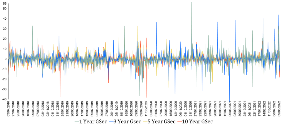
Figure 1 below presents a chart of the daily yield change in these 4 securities over this entire period of little over 4 years and 993 trading days.

Figure 1: Daily Change in Yields on GoI Securities in Basis Points